In precedent with my other Substance Nodes, this blog will accompany the Histogram Equalization node. It will be a two part series going through the node; how it works from underlying theory to Substance Designer implementation.
NOTE: Adobe has implemented histogram equalization natively into the program since writing these posts.
First we will discuss histogram equalization, then in part two, we will cover the Substance Designer implementation.
If you don't know what it is, you can think of it as a kind of contrast adjustment for an image. Somewhat like doing an levels adjustment or using the existing histogram nodes in Designer.
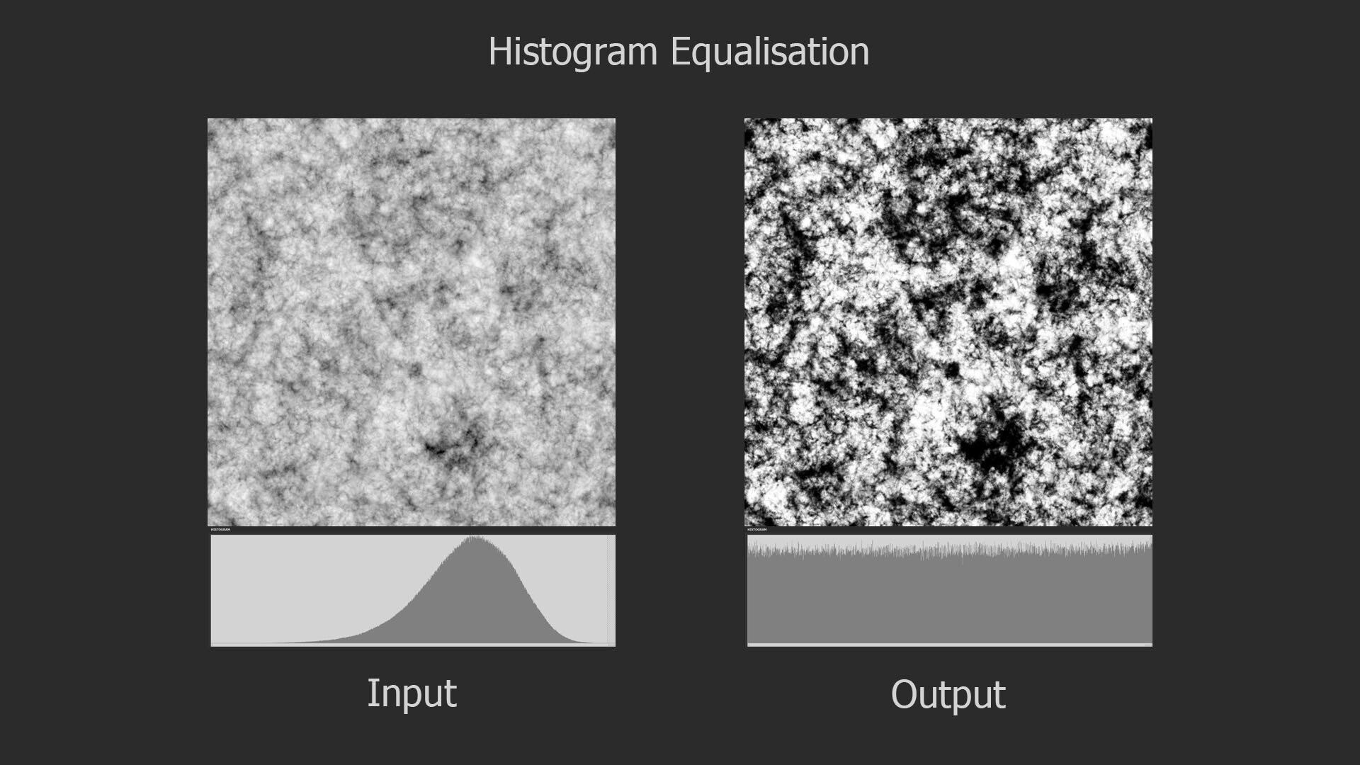
However, equalization is actually something quite different. Here is a more formal definition: Histogram equalization is a technique used to redistribute the intensity values of an image so that they are uniformly spread across the available range (typically 0 to 255 for an 8-bit image). The goal is to make the histogram of the modified image as flat as possible, meaning that each intensity value is equally probable.
If any of that did not make sense to you don't worry, hopefully it will by the end of this post. So lets begin with understanding what a histogram is exactly and why we might want to equalize it.
A histogram is a graphical representation of the distribution of pixel values within a texture. The x-axis shows the range of pixel values, and the y-axis is a count of how many pixels had those values in the image. Visually, a histogram is often used to understand the characteristics of a texture, such as brightness or value range. Programmatically, a histogram is often used to analyze and adjust the contrast, brightness, and overall tonal balance of the image.
For our histogram below, these values are grouped into 20 evenly spaced 'bins' for easier viewing (but is it common to use 256). Then each pixel value which falls into a bin, is counted.

If you divide the histogram counts by the total number of pixels in the image (a process known as normalization) and draw a continuous curve through the points, this is called a Probability Density Function (PDF). The PDF tells you the probability of a pixel having a particular value.

While a histogram provides discrete counts, a PDF gives you a continuous probability curve, a subtle but important difference. In the context of everyday 3D art and textures, they can be used interchangeably, but it's important to understand the subtle differences between them since one speaks about counts and the other probability.
If you have spent any time with Substance Designer, you have likely seen the histogram. Typically we use nodes like histogram range or auto levels as a way to manipulate it, however unlike those nodes, which are linear operations (meaning your just moving the histogram up, down or stretching it), equalization completely redistributes the values in the image, changing the profile of the histogram itself. In the image below, notice how the linear operations maintain the bell shaped hump in the center, while the equalization changed the profile completely.

In the context of texturing, this can be incredibly helpful for all kinds of things. A common use case could be for generating color information with a gradient map or my color nodes (shameless plug). Equalizing the input image will ensure that you sample the full range of colors and not bias it to a small region of the color gradient.

If you cumulate the histogram, by going through each bin, summing the count from the bin before, you create what is called a Cumulative Distribution Function (CDF).

This function represents the probability that a pixel will have a value less than or equal to a given number. Unlike a Probability Density Function, which shows the probability of a pixel having a specific value, the CDF shows cumulative probabilities. It is not often you will come across a CDF in day to day texture work, but in the context of image processing, this information can be very useful and as you may have guessed, it is crucial for performing histogram equalization.
Lets look at some histograms to familiarize ourselves with how both PDF and CDF looks for difference types of images.
In the image below, we have a relatively mid tone image where most of the pixels are floating around the mid range. Notice how you can see this behavior represented both in the PDF with its hump in the center and the CDF transitioning sharply in the same location.
In the next image, the values are mostly residing in the upper range, which moves everything up in the PDF and CDF also.
While a darker image pushes everything to the lower range.
One very important PDF/CDF is that of an image where every pixel is equally likely. Such as a linear gradient.
Notice here that each histogram bin has exactly the same count, thus each pixel value has the same probability of occurring, which in turn means the CDF is a perfectly straight line. Why this is the case is essential to understanding equalization, so take a moment to think on it if it feels ambiguous. Here the CDF is saying that each pixel value (x axis) has the same cumulative probability (y axis). Or, put in other words, by half way through the value range (x axis), I will have seen exactly 50% of the values (y axis). Or, by value 0.75, I will have seen exactly 75% of the values and so on.
Histogram equalization works by remapping the image pixel values according to its CDF. What that means in practice is computing a CDF for the image then replacing each pixel value with the corresponding CDF value.

If you were like me, this seemed incredibly simple, but also...what?! Sure, remapping pixel values is straightforward (gradient dynamic node in Substance), take one value and convert it to another based on that function, but it was not at all clear to me why remapping with the CDF would work, much less one generated from the image itself.
To better understand this, consider the transformation as a function, let's call it f(x). In this equation, x is the input image, and the output we want to be the remapped equalized image. It's logical to assume that f(x) would be related to probabilities, after all we are trying to equalize the image and the CDF does indeed provide a probability distribution for the image. But still, it wasn't clear to me why this works. I did not have an intuition or clear visualization of what was happening.

Recall, the CDF tells you the probability that a randomly picked pixel will have a certain intensity value or lower.

When remapping, I like to visualize it as projecting that CDF curve onto the x=y line. This line also happens to be what a perfectly equalized image CDF looks like, as we saw before.

This projection is essentially saying something like "we want 80% of the pixels to have occurred by value 0.8, not 0.27 which is where it was before". This is why using the CDF works, its taking all the probability information in the image, and forcing it to be linear.
That's all there is to it really. It is a single remapping from one set of values to another but all the mystery and magic comes from those set of numbers containing information about the pixel value probabilities.
And that concludes the first part of our jump into histogram equalization, I hope it was useful. In the next part of this series, we will go through how this can be implemented in Substance Designer.