Welcome to part 3 of my development blog! This is a continuation of the last two posts, so make sure to read them if you haven't yet!
Part 1
Part 2
In the last post we discussed using a circular kernel and explored different sampling patterns. We had moved away from using a stride value and instead defined a maximum search radius and scaled the sample points with that. However, textures with large variation in shape size will have problems as the search radius increases. In fact, we loose smaller shapes entirely, due to the radius becoming larger than the shape itself.

So what if we could scale this radius value per shape? In case you are not aware, the flood fill to bounding box size actually outputs a normalized size for each shape. Exactly what we need.
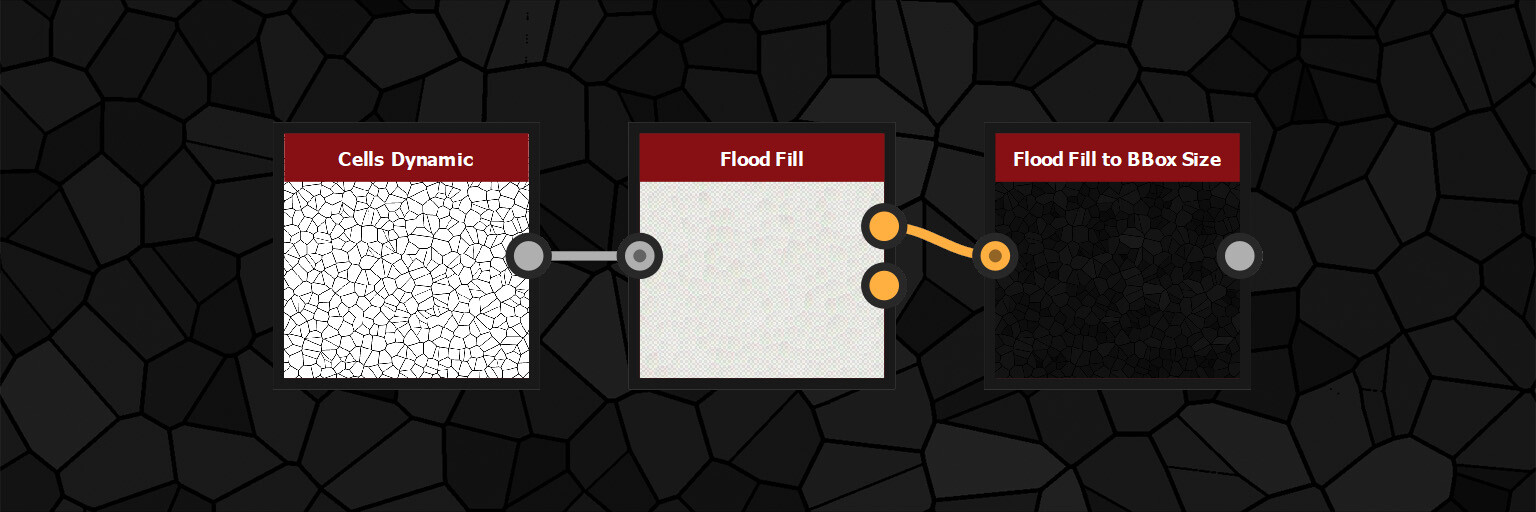
The values in the map are normalized to uv space, meaning if we multiply them by the texture size, they will actually give us the bounding box size of each shape in pixels!
If we were to then scale the search radius by this bounding box size, our kernel would then respect each shape individually.
Of course, the bounding box size is going to be different for the x and y axis, so lets take the largest number of the two, max(x, y), as a start. This is also the default on the flood fill to bounding box node.
Left is without dynamic scaling, right is with.
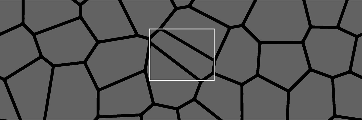
A big improvement already! However, a lot of the shapes are still becoming very small or disappearing again. This is due to the bounding box not accurately representing the shape in question.
Diagonal thin shapes being the worst offenders. Notice how poorly the box fits around the shape.
The flood fill to bounding box node has two other outputs, the values for x and y values respectively. Maybe we can get a more accurate bounding box by averaging the two, rather than taking the max. The image below shows a comparison between max(x, y) and (x + y) / 2. Green denoting how much we have improved.
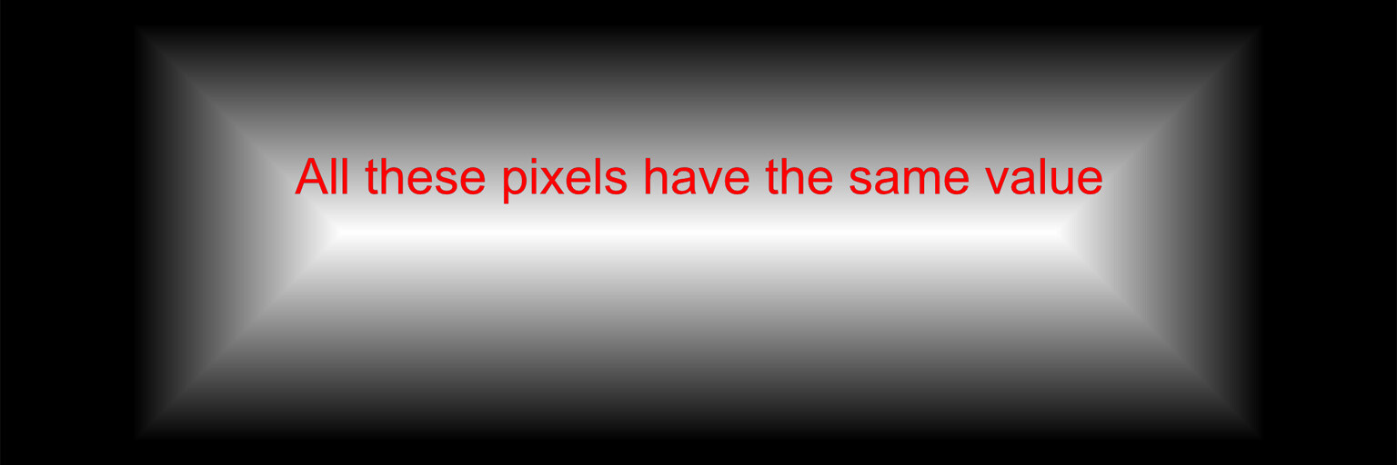
Another good step forward but we are not quite there yet. Some shapes are still disappearing. After consulting with my lead again, he suggested I look into calculating the largest circle that fits inside the shape. In fact, the distance node can be used to generate this value. If we set a value of 256 on the distance node, it produces a full 0-1 gradient the width of a texture, regardless of the size. In the image below, we have a single line of pixels on the left and a distance node set to 256.

This is incredibly useful. If we were to distance our shapes, then the brightest pixel in each shape would actually be representing the largest radius that fits in that shape, in uv space. (I have made the image brighter so it is easier to see).
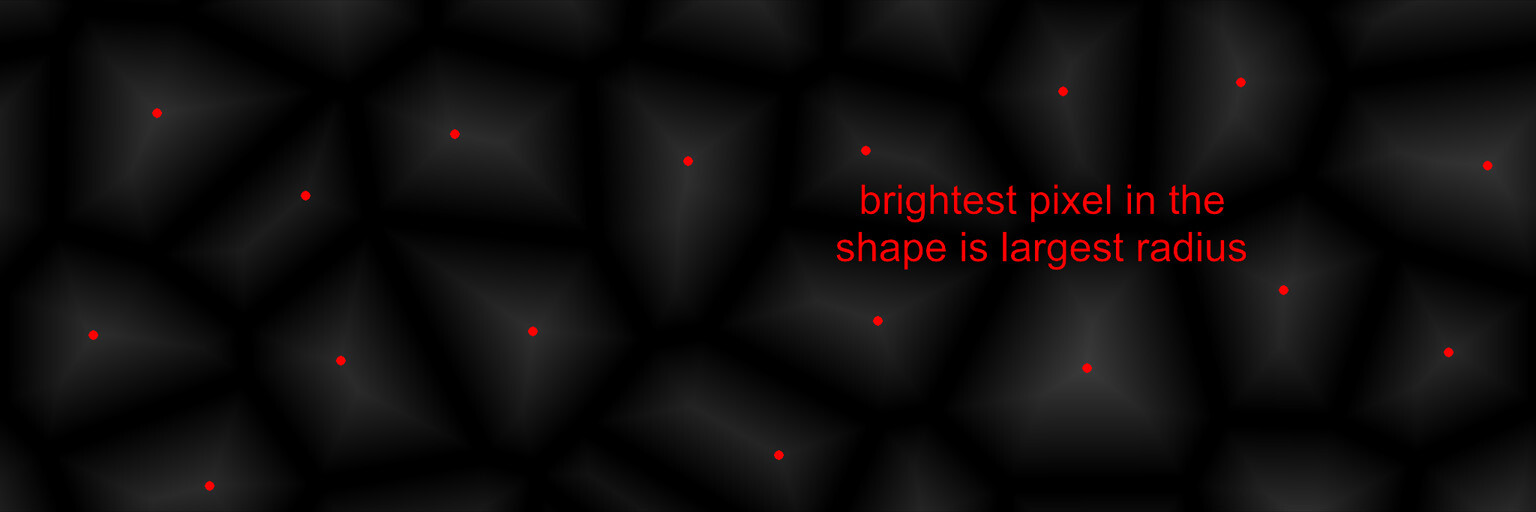
If we know the largest radius in a shape, that is the same to say we know the largest fitting circle.

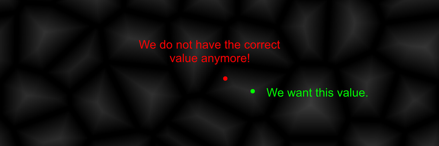
That looks like a pretty good maximum search radius for our sample points to me! But, how do we get access to that value? It's not like we can simply plug the distance node into our pixel processor as the search radius is calculated per pixel. In the image below, our radius value would be wrong if we were currently calculating the red pixel.
What we need is that radius value dilated within each shape. Perhaps we can use the flood fill to grayscale node? Again, I have brighten the image to make it easier to see, but this is the flood fill to grayscale blended with the distance on max(lighten).
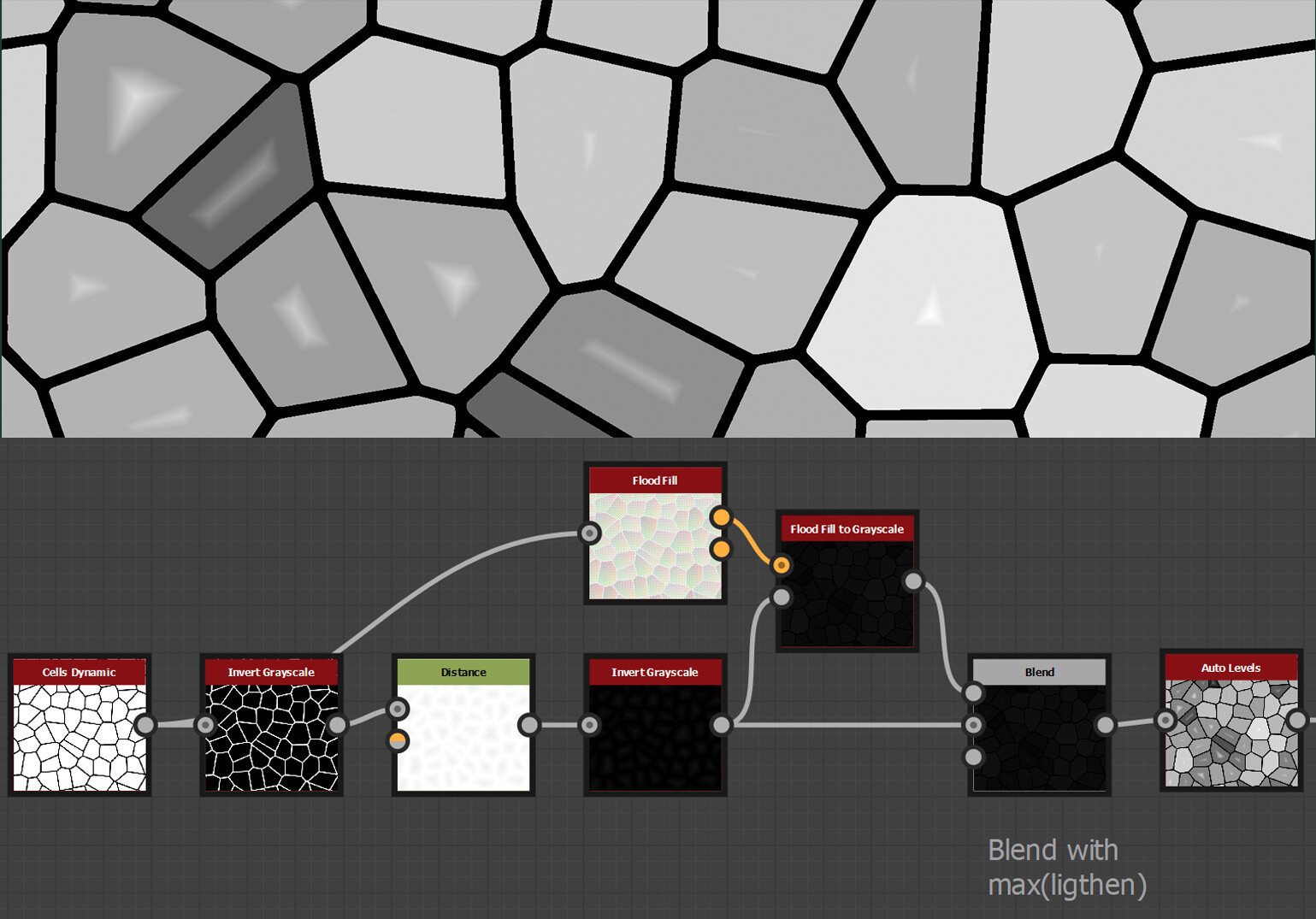
This was close, but you can see the flood fill to grayscale is not finding the brightest pixel and therefore dilating the wrong value. This is because the brightest pixel could be in any arbitrary position in the shape, and most certainly not the one the flood fill to grayscale is choosing.
Perhaps we can isolate the brightest pixel and dilate from that position instead? I thought maybe the easiest way would be to find the local maximum value, another neat idea from my lead. (poor guy has to listen to all my designer problems).
We wont go through the details of local maximum here because it didn't work out very well. But as a high level, it works similar to the blur we implemented. Except rather than averaging the kernel, we check to see if any of the neighbors are brighter than itself. Which means it will only output a white pixel at the very peaks.
Regardless, as you can see in the image below. Some cells are missing and I was not able to consistently produce a pixel at the peak of each shape.
I think this was largely due to the shapes potentially having more than one pixel with the brightest value. Like a rectangle for example.
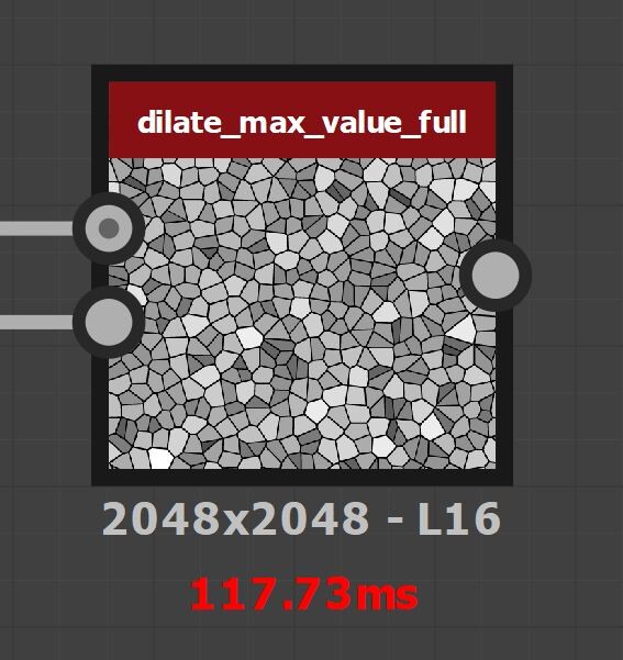
So, what if we just create our own dilation node instead? We could take a 3x3 kernel again and simply output what ever is the brightest value. Of course, checking the shape ID's as usual.

Do this enough times and we will have dilated the brightest value! This is with 50 something passes.

But, how many passes is enough to fully dilate an image? Well again, this is resolution dependent, and different for each shape. Since designer doesn't support loops, our only option would be to assume the worst case and dilate the same number of times as the texture size.
Honestly, after a couple of hundred passes, the performance was so bad I just stopped.
Ok, so this wont work. It was Ole Groenbaek whom I was complaining too this time and together we went through the flood fill node looking for inspiration. In here we found a neat trick for cheaply dilating the value we need.
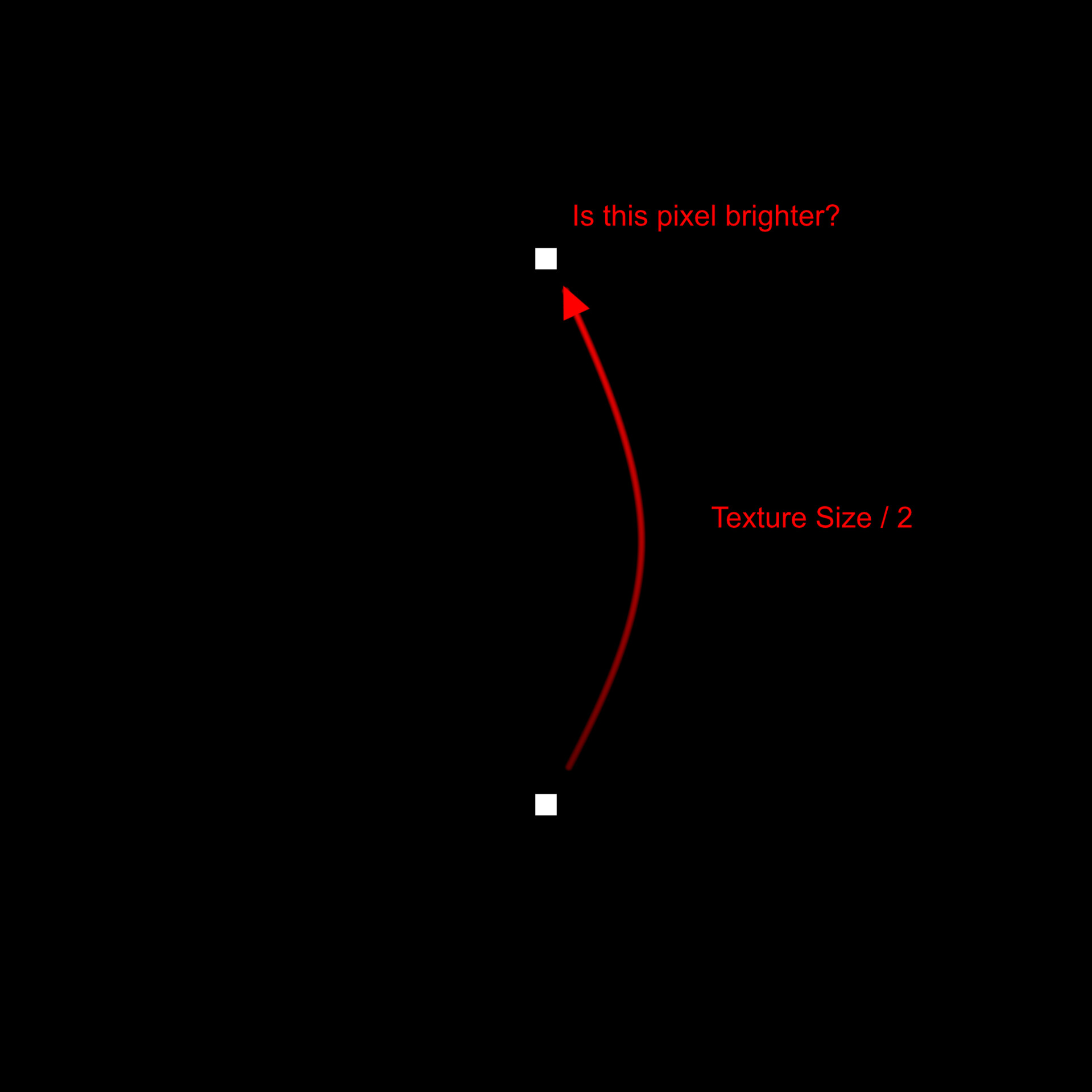
Say we have our pixel whose value we want to calculate. Rather than looking at the neighboring pixels, instead we look at a pixel exactly half the texture size away. If that pixel is brighter, we change our one, otherwise ignore it.
We then repeat this process, except this time we look half way between the first two.
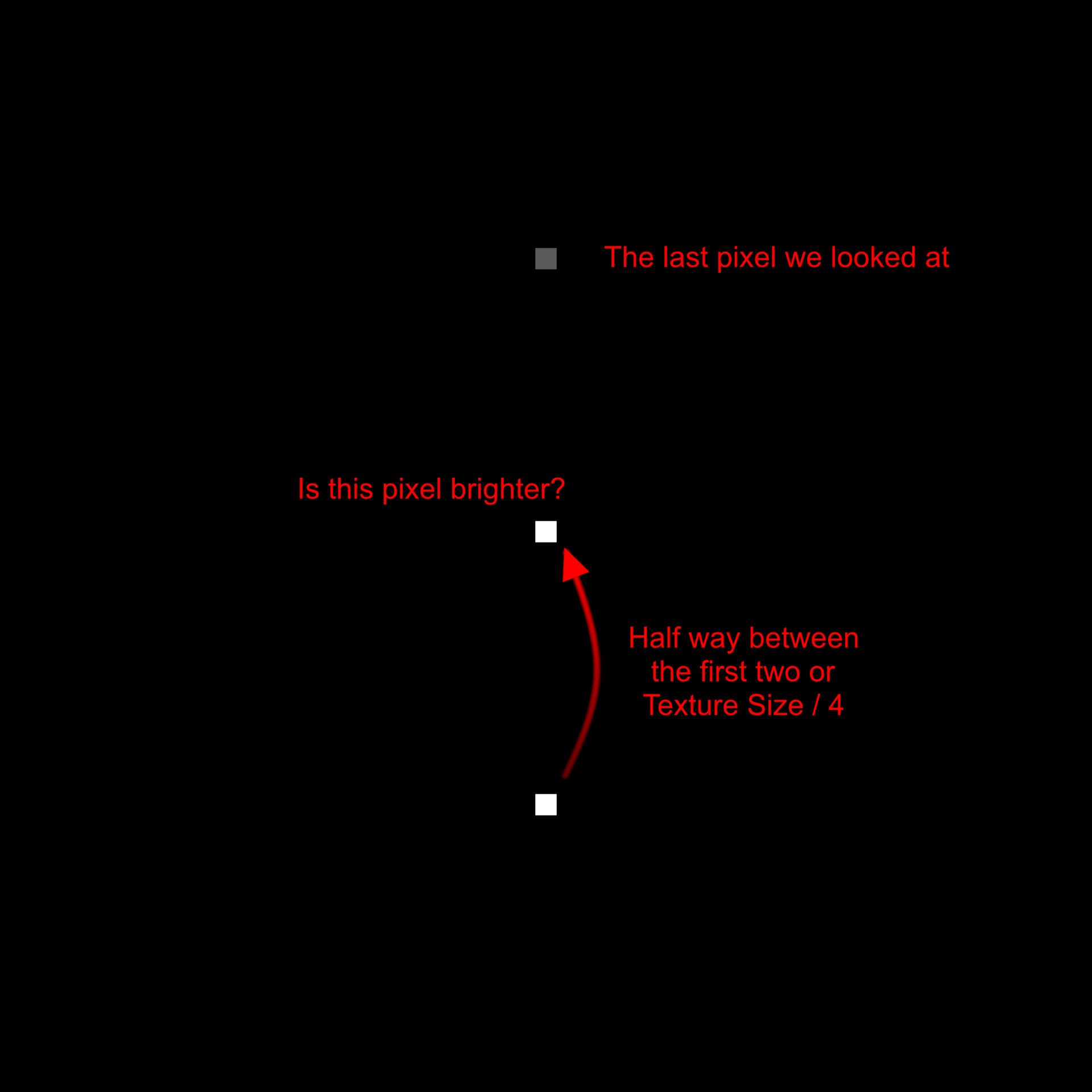
And repeat, each time looking exactly half way between the last until we have filled out a full line.
What we are doing here is actually stepping down the texture resolution each time, meaning we only need to do a maximum of 12 passes should we want to fill a full 4k image. If we do this process on our image, checking the cell ID as usual, we have cut down the number of passes needed tremendously. In this example, there are 11 passes (to fill a 2k image) and instead of doing it up-down, we do it for each diagonal axis. (This was because I found it worked better with the typical cell shapes).

You may notice that some cells still have a gradient at the corners however. So for this reason, I repeat this process a second time, just to be sure all values are fully dilated.
What we have actually done here, is sort of half implemented a version of the jump flooding algorithm. Something Igor Elovikov pointed out to me after releasing the node. Jump flooding is exactly the process described above, but rather than looking at 1 pixel at a time, we look at 8.
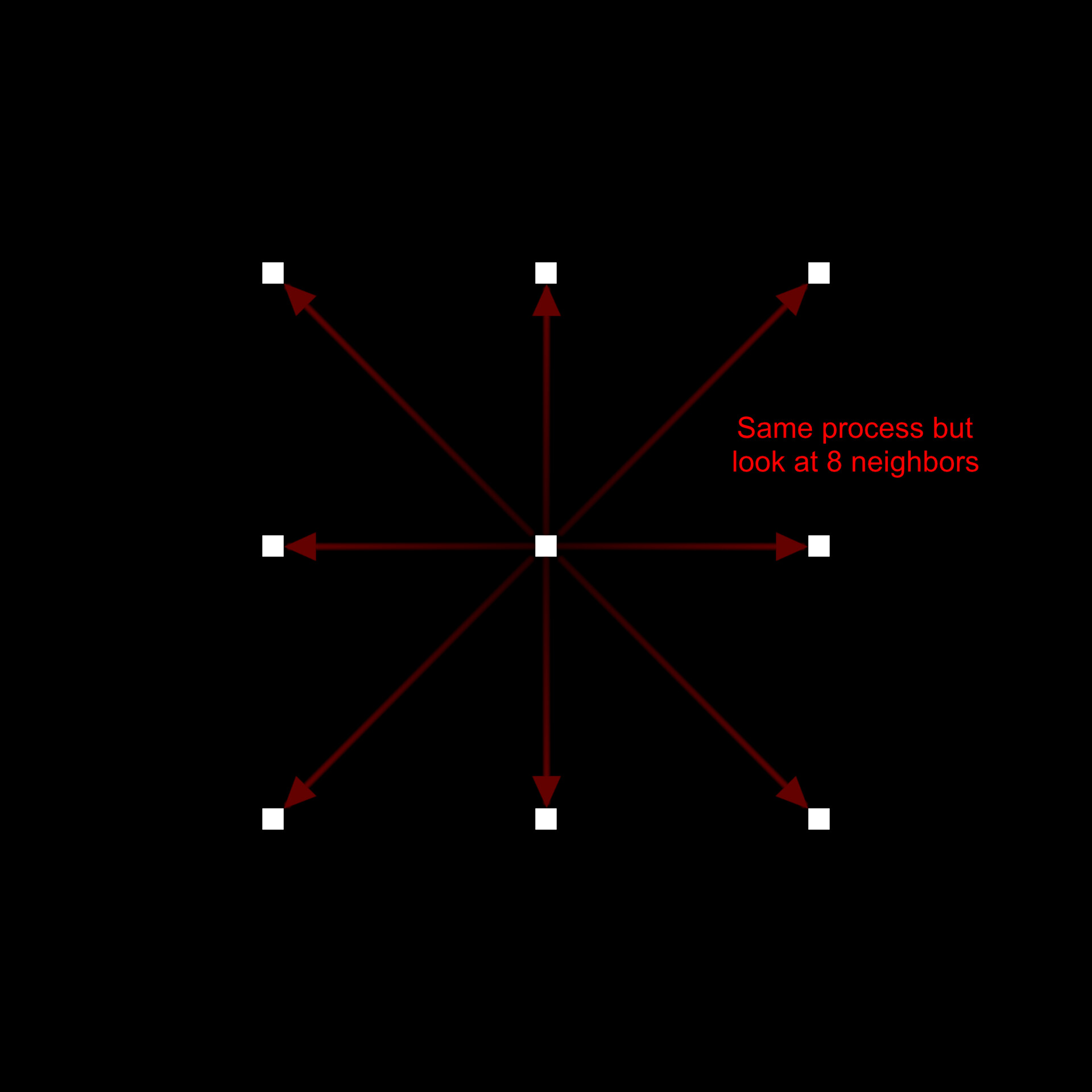
This offers all the same benefits, is more accurate and it is cheaper since we end up doing even fewer passes in total. My reason for not using jump flood is simply because I didn't know about it, nor did it occur to me we could do the same process with 8 neighbors at a time.
I wanted to draw attention to this though, as it is absolutely the way to go, should you implement anything like this in the future.
With this, we have our largest fitting circle radius which we can scale our kernel by.
Even with my best efforts to reduce performance cost, the node was still ranging from 20ms (on the lowest settings) up to 70ms (on highest) on my GTX 980 card, so I didn't want to have this feature on by default.
In fact, it does such a good job of preserving the shape, that some just looked strange.
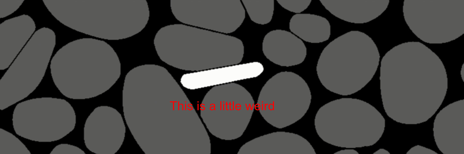
Perhaps we should add a slider to let you transition between bounding box and best circle fit scaling.Which as it turns out, visually feels like your pruning smaller stones or not.
As a final optimization, when the slider is 0, there is a switch to disable the best circle fit calculation.
With these changes, our kernel search radius now depends on an input map.

This means the kernel is actually calculated per pixel, which in turn means we can manipulate it to produce some very interesting shapes. What you see below is the search radius being scaled by an additional variation input map (Which is animated for the gif).
This was another feature I had overlooked until Stan Brown suggested it to me! A good thing too since it was trivial to implement, only taking an additional multiply, and gives rise to much more flexibility in the node.
That concludes this series about the development of the node. I hope it was interesting to read and you are left with a good understanding of how the node works. As I mentioned in the first blog, I am sure there are better ways to create something like this. But regardless, it was a very enjoyable experience for me and so I wanted to share that with the community.
Thanks for reading everyone!