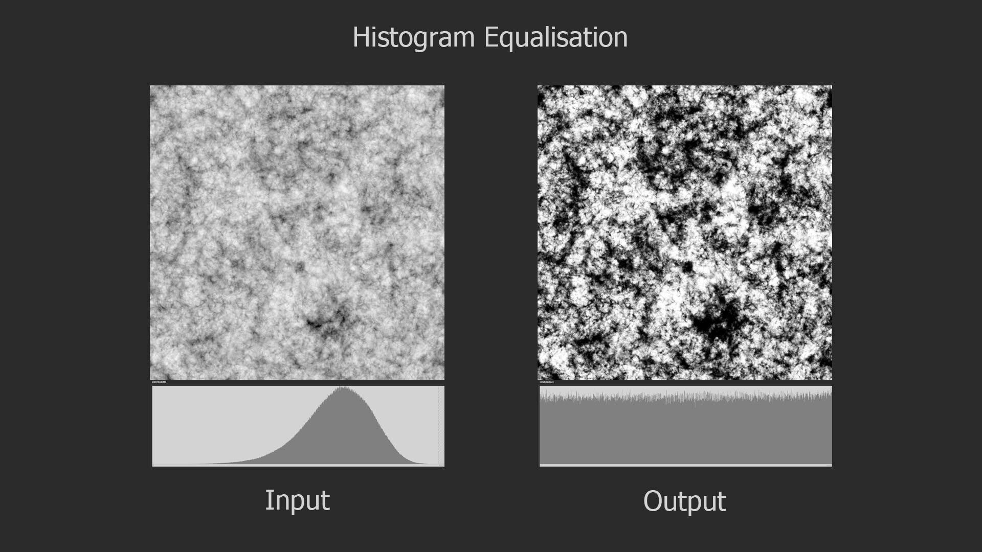
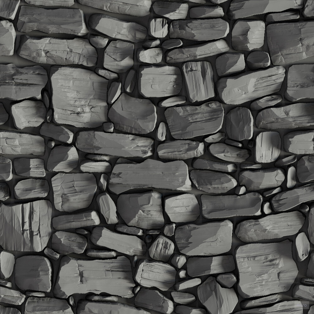
In my last blog post, we explored the fundamentals of histogram equalization. If you have not read that yet, you may want to do so first as this post is a direct continuation of that. Here we begin the practical implementation in Substance Designer itself. Initially, I planned to cover the entire process in one go, but due to its complexity, I've decided to break it down into segments. So in this installment, we'll focus exclusively on computing the Probability Density Function (PDF).

I will assume you have some familiarity with Substance Designer's FXMap, as I won't go into its basics here. There is simply too much to cover about the node and CGVinny (who works at Substance) has done great resources on that topic already. My aim is to provide us with a clear understanding of PDF computation and a visual understanding of the function graph itself. While knowledge of the FXMap isn't critical, it will help. So, let's get started.

The histogram equalization node consists of three main components: PDF computation, Cumulative Distribution Function (CDF) computation, and value remapping. We will focus on the PDF node.

While the actual node you can download contains multiple setups for varying bin counts, we'll simplify things here by focusing on a 16-bin example. Trying to visualize and animate more than 16 is difficult! In the downloadable node, you'll find four different bin configurations: 64, 128, 256, and 1024 bins. However, the computational approach remains the same across these variations.

Probability Density Function (PDF) in Designer

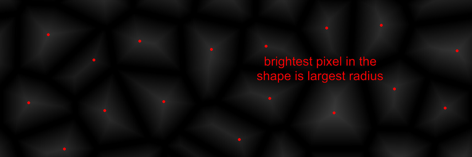
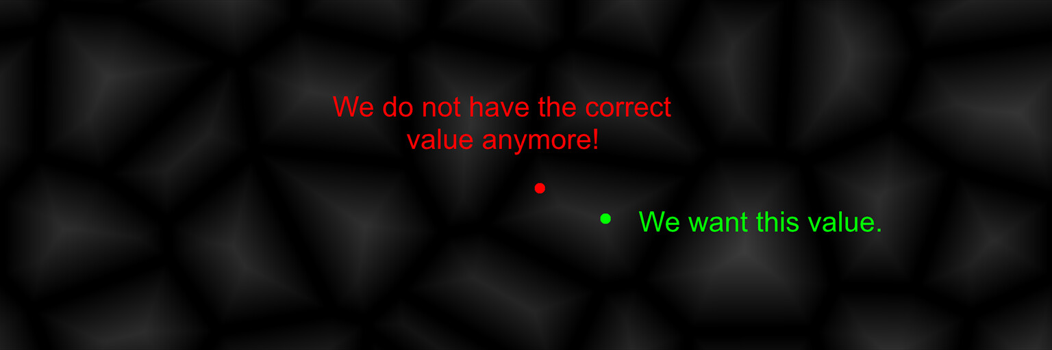
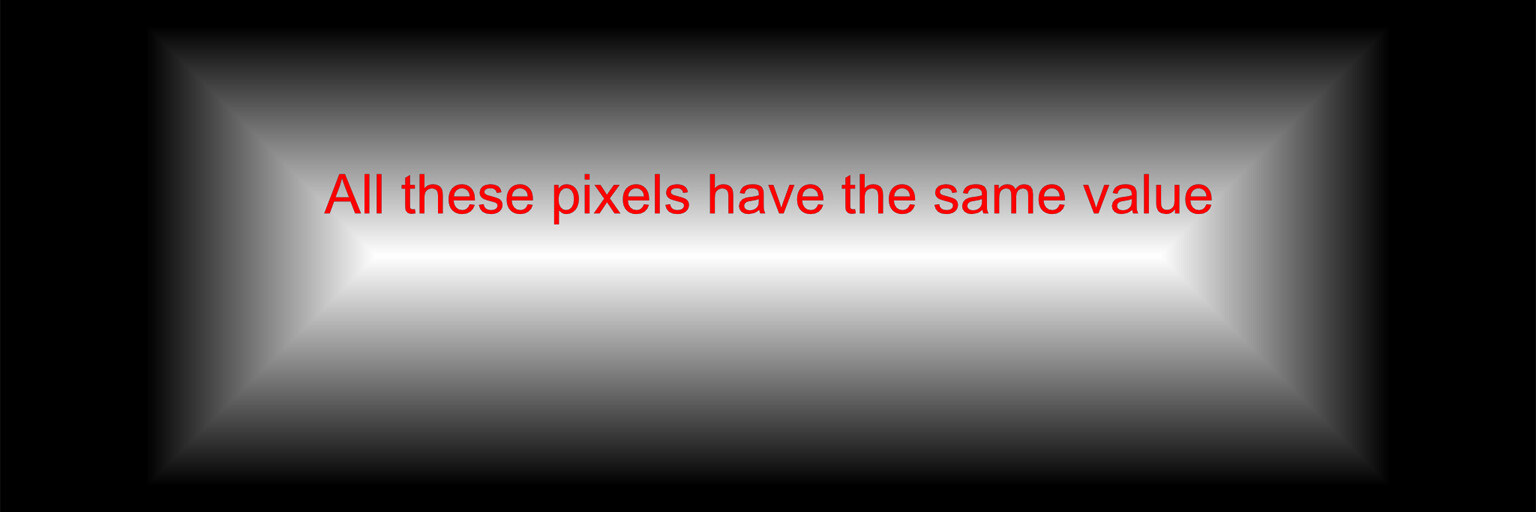
If you recall, the PDF represents the likelihood of each pixel intensity value appearing in the image. We previously saw this as either a graph with bars or a continuous function but in Substance Designer, we don't have those representations available to us. Instead, we need to store it as a 1x16 image, with each pixel's value corresponding to the probability of its respective bin along the horizontal. The entire goal in this post is to generate this 1x16 image. We are aiming to eventually build a Look Up Table (LUT) that will remap our original pixel values to the Cumulative Distribution Function (CDF) and this is pixel strip containing PDF values is the first step in that. In the released node, this means generating a 1x64, 1x128, 1x256, and 1x1024 image respectively.

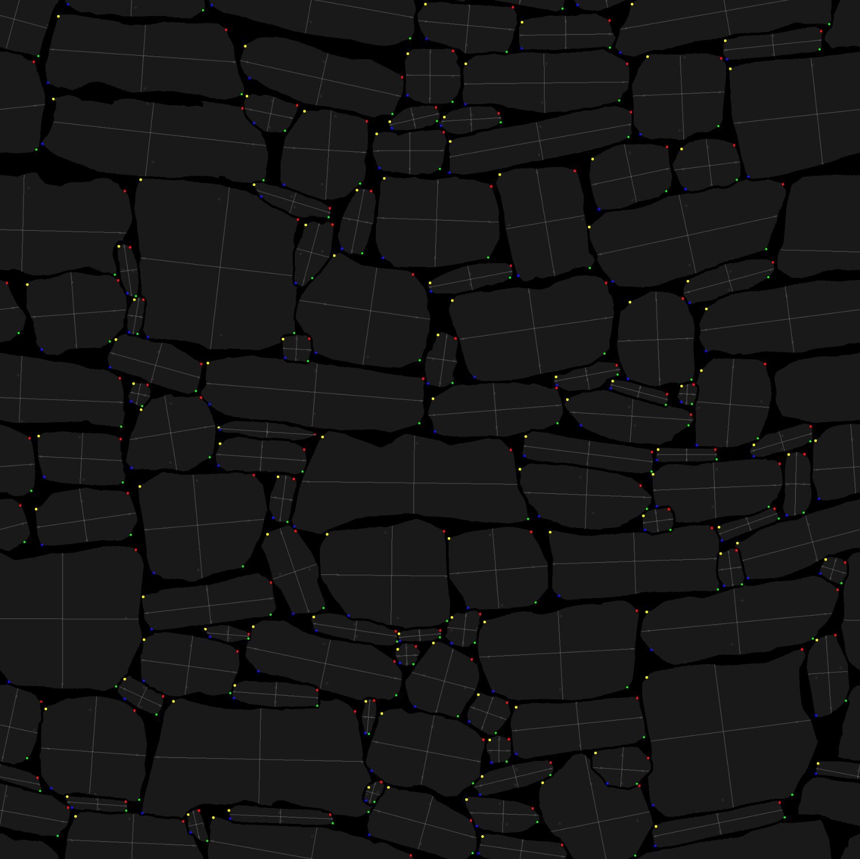
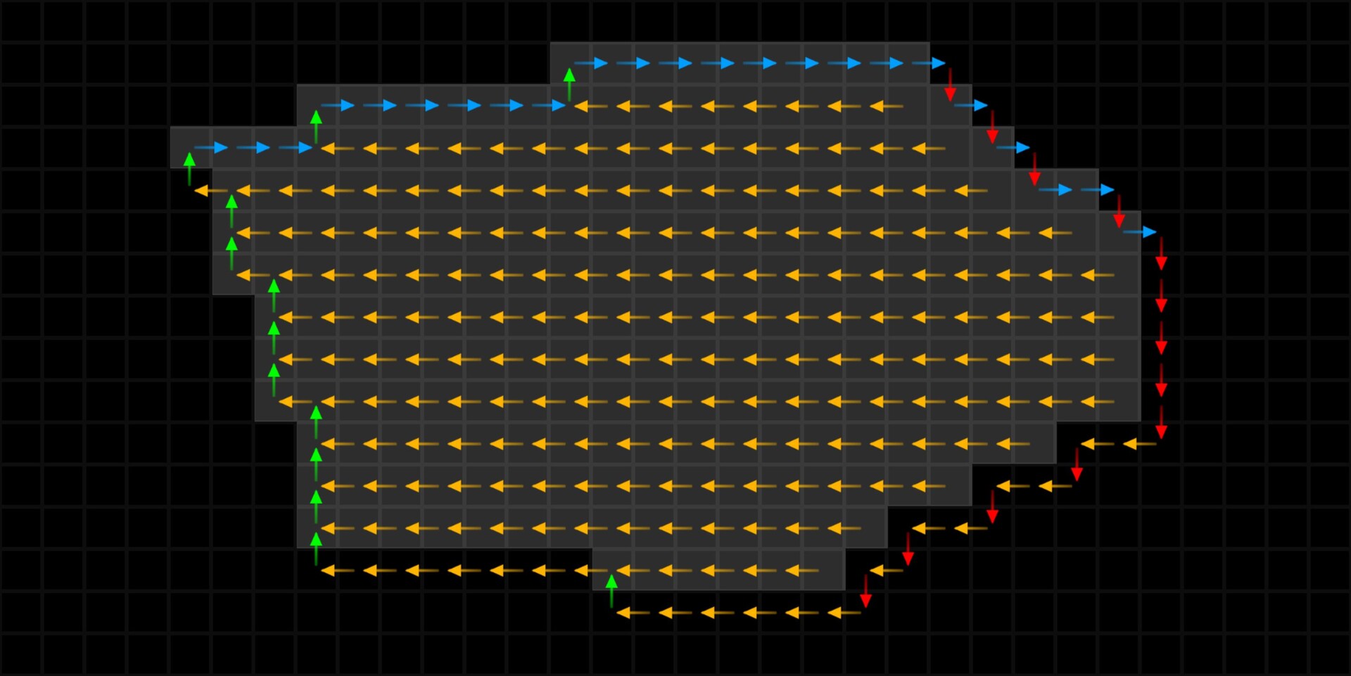
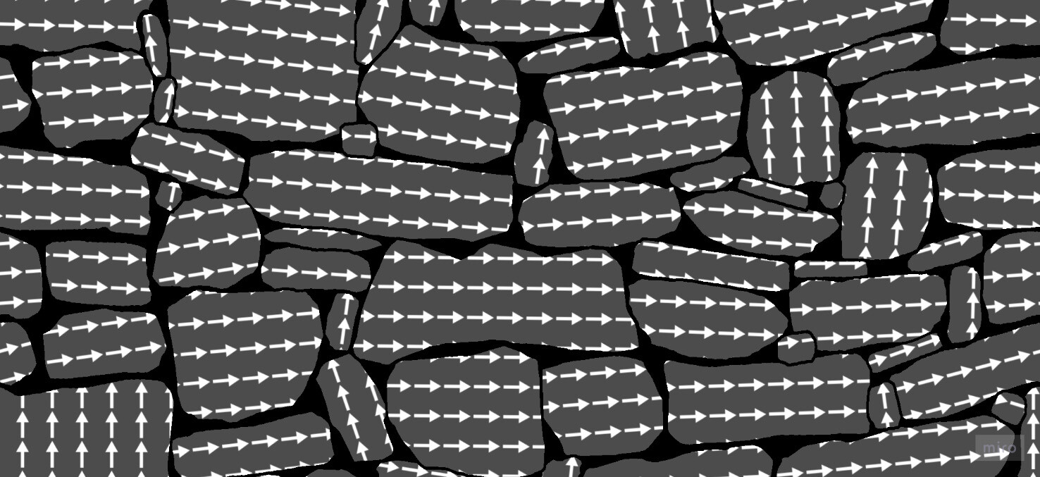
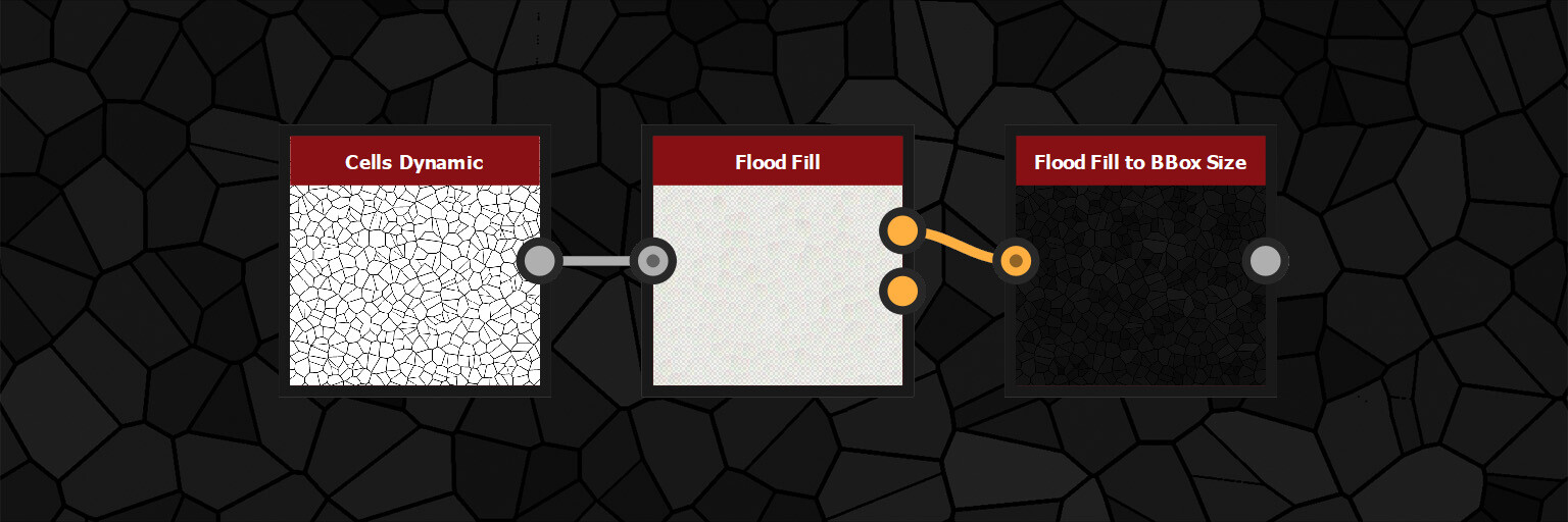
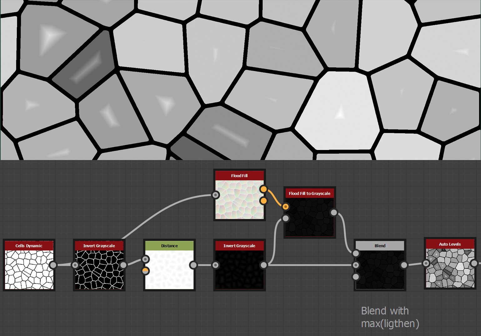
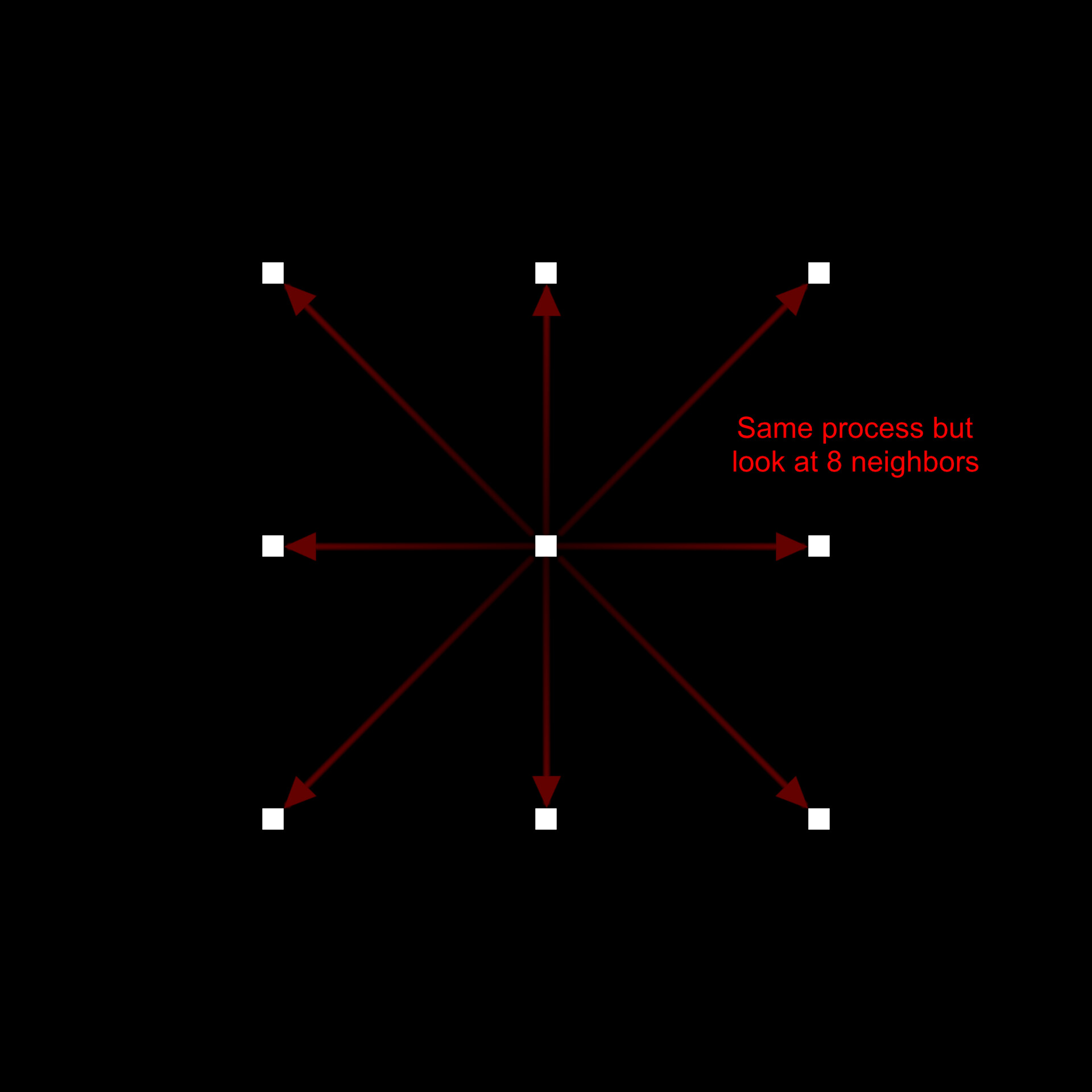
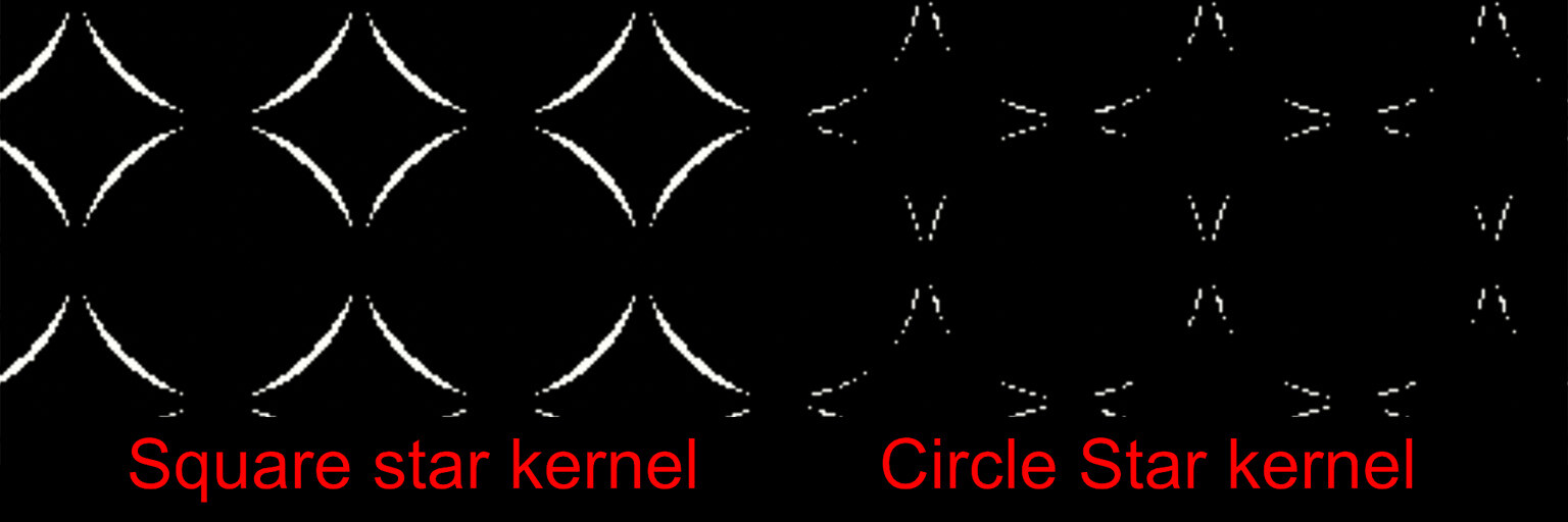
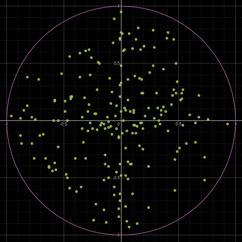
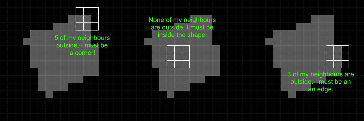
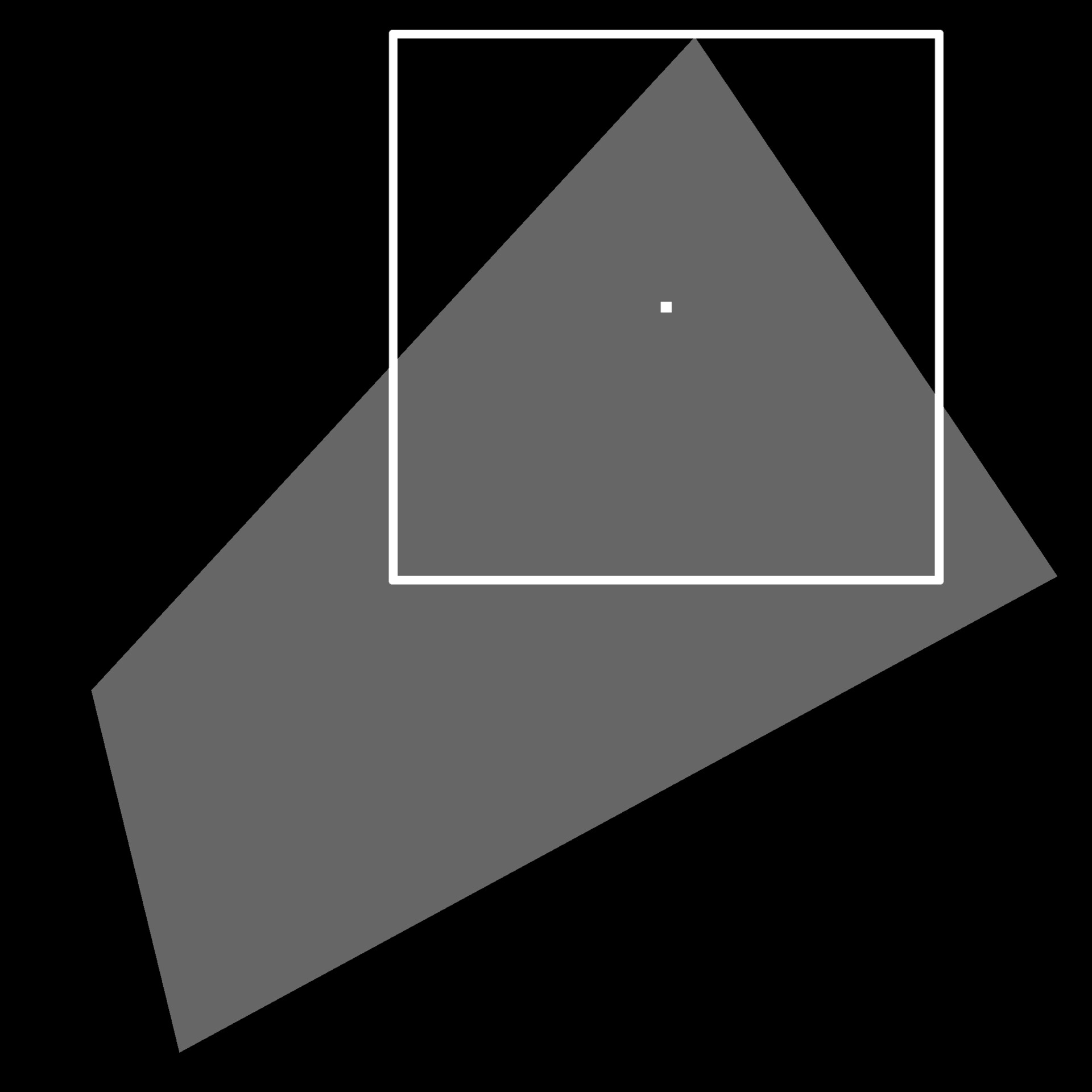
To generate our PDF, we use the FXMap, connecting multiple Quadrant nodes to subdivide the image into 16x16 squares. These squares serve as our 'samples'. Using their coordinates, we sample the image pixel values, which are then categorized into bins and counted to produce our PDF image. Sounds confusing in words but check the animation below. The process will work like this:

• Sub divide: Image will be sub divided into adequate resolution.
• Sampling: Use the sample position to get the pixel value at that location
• Value binning: pixel values will be modified so they fall into a bin.
• Bin assignment: Samples are moved into a new designated bin location along the horizonal
• Aggregation: Samples with identical pixel values end up in the same location, making counting straightforward.

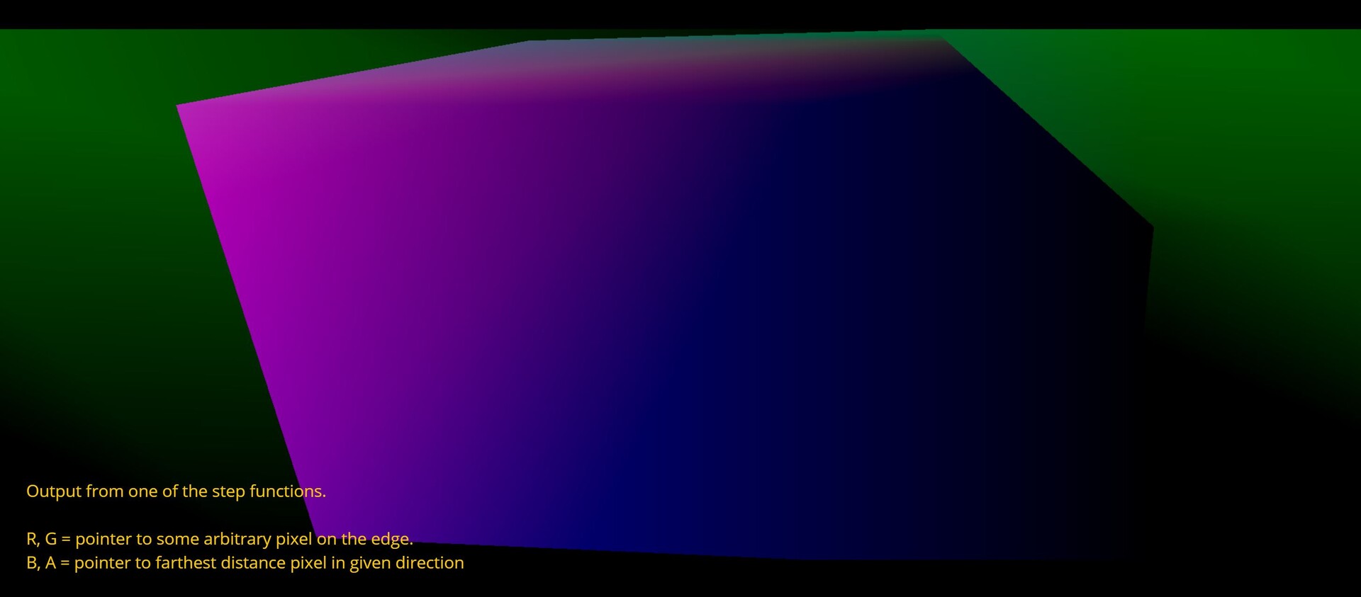
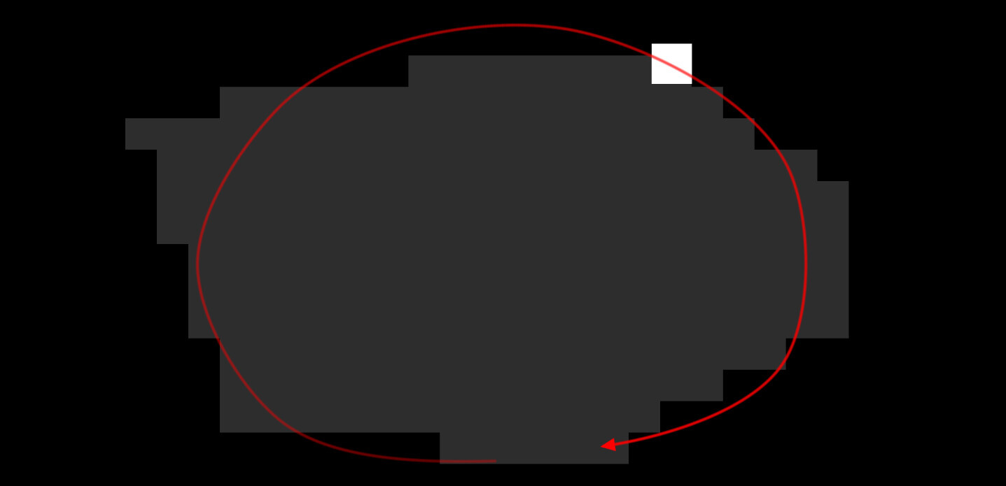
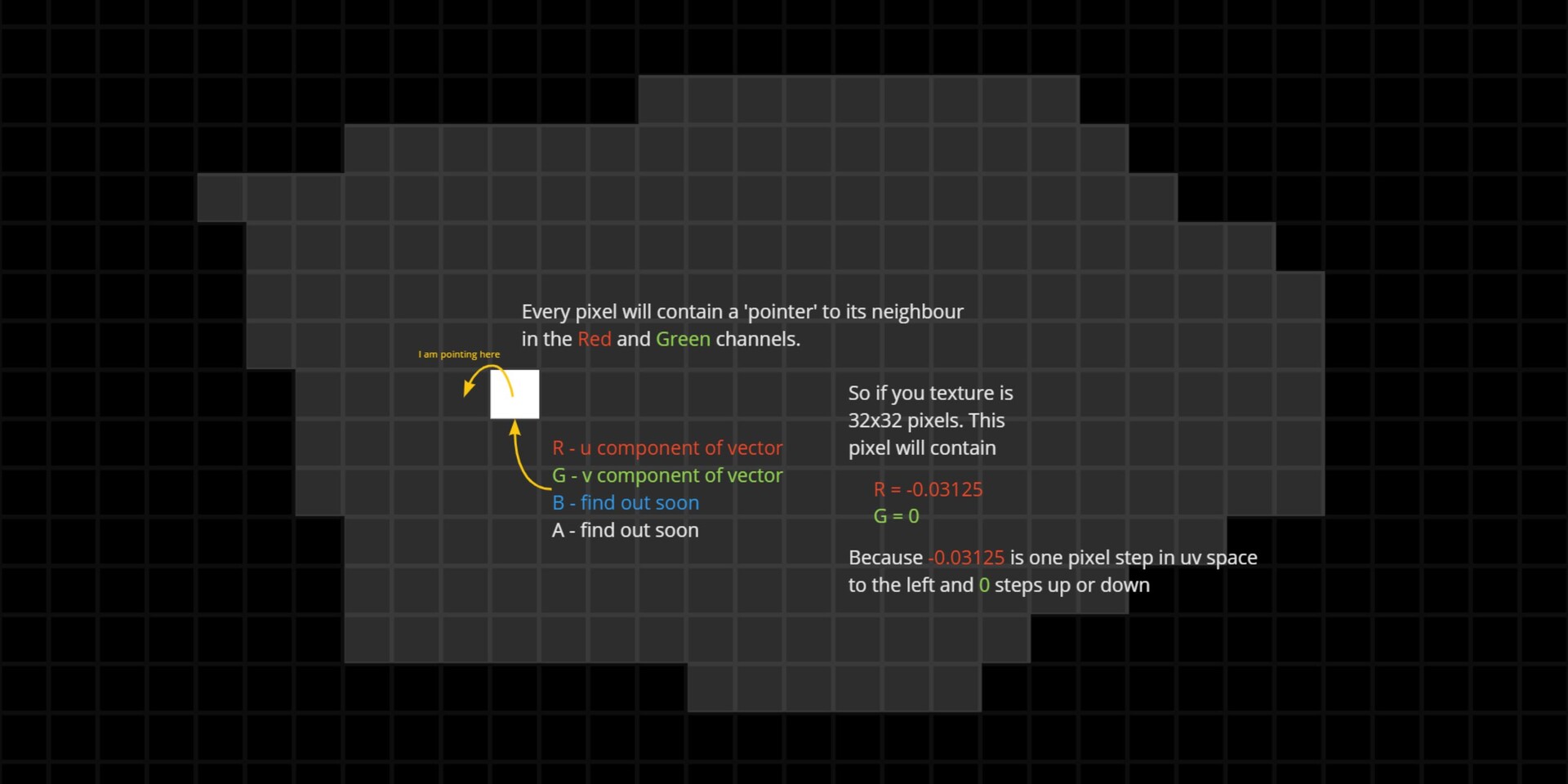
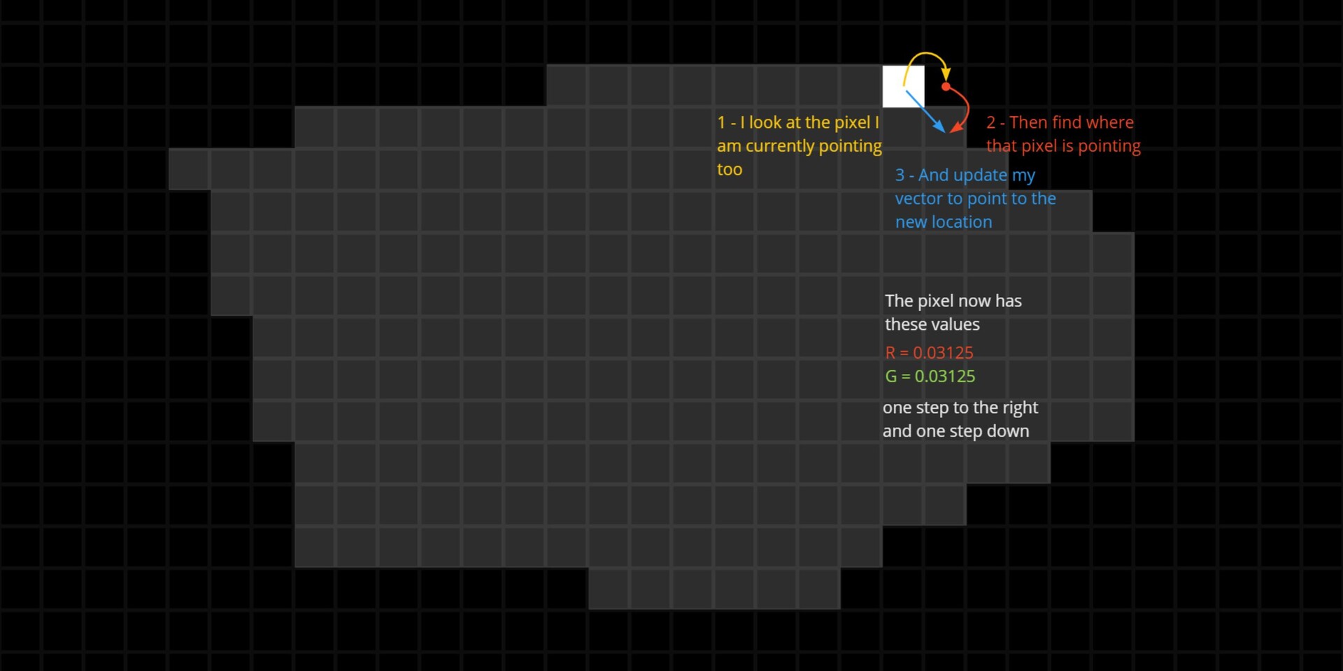
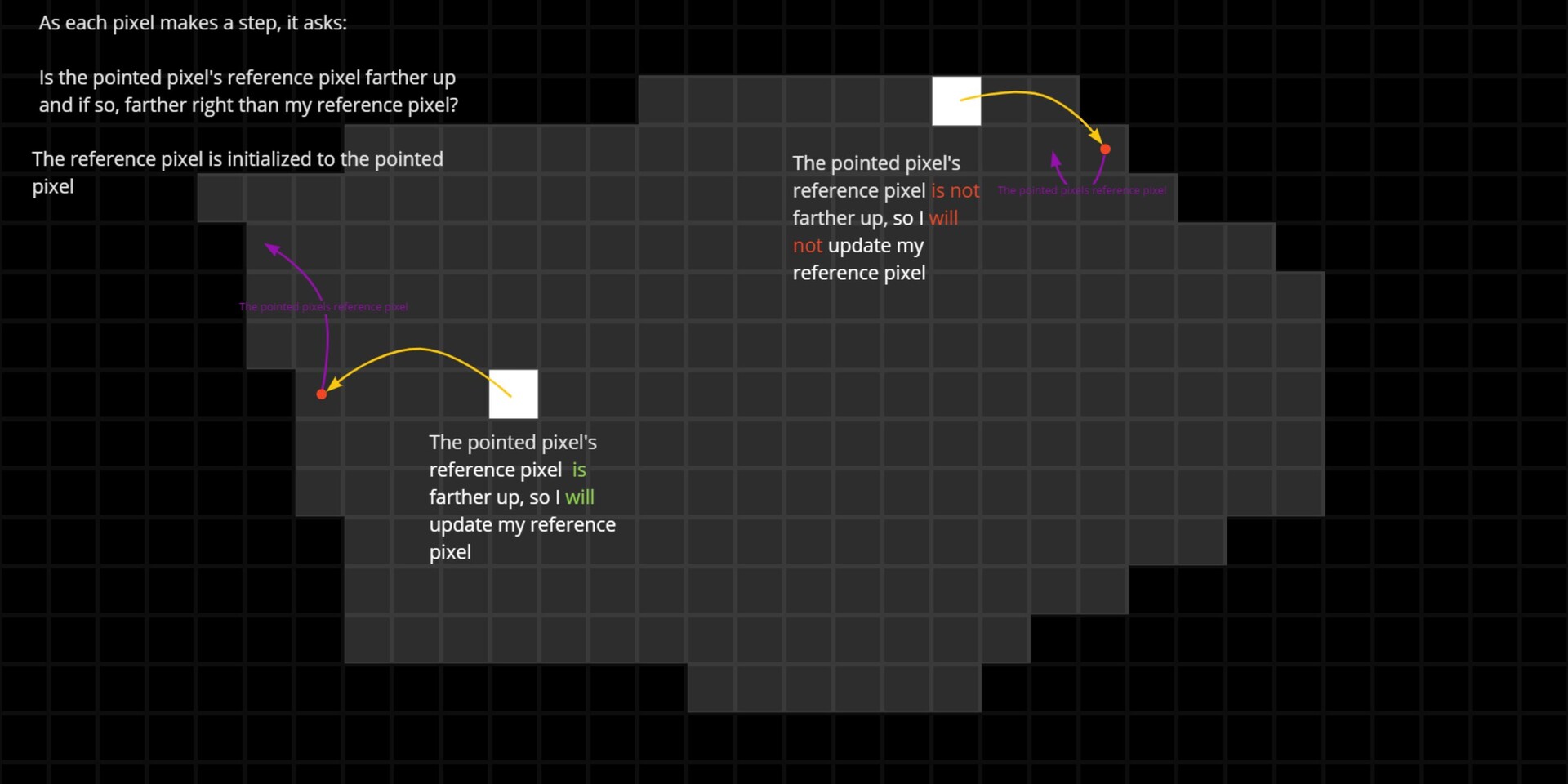
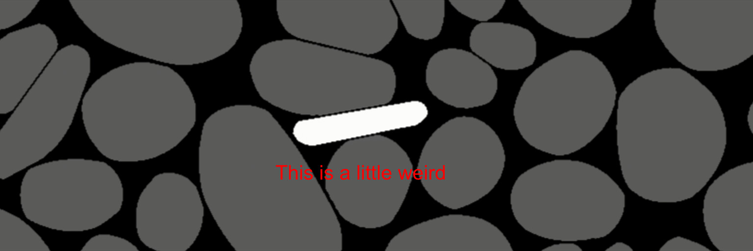
To actually count the pixels, each sample in the image will be repositioned based on its pixel value. This repositioning moves a sample into a predefined location, somewhere else in the texture, with the idea being that samples with the same pixel value will move to the same location, providing us a means to count them. We can have the bin locations next to each other running horizontal, starting from pixels with a value of 0 through to 1. While the animation below shows the strip to the right, it will actually be placed at the top of the image, which you will see shortly.

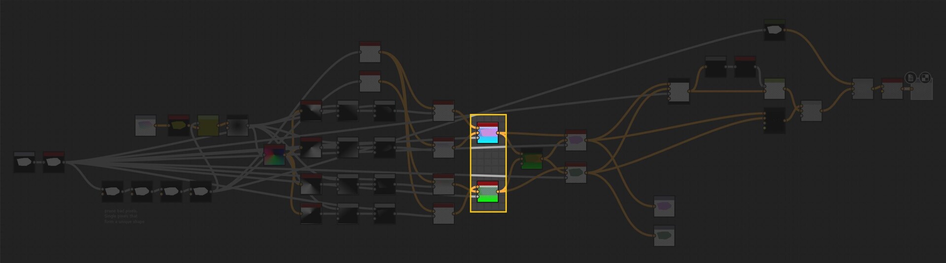
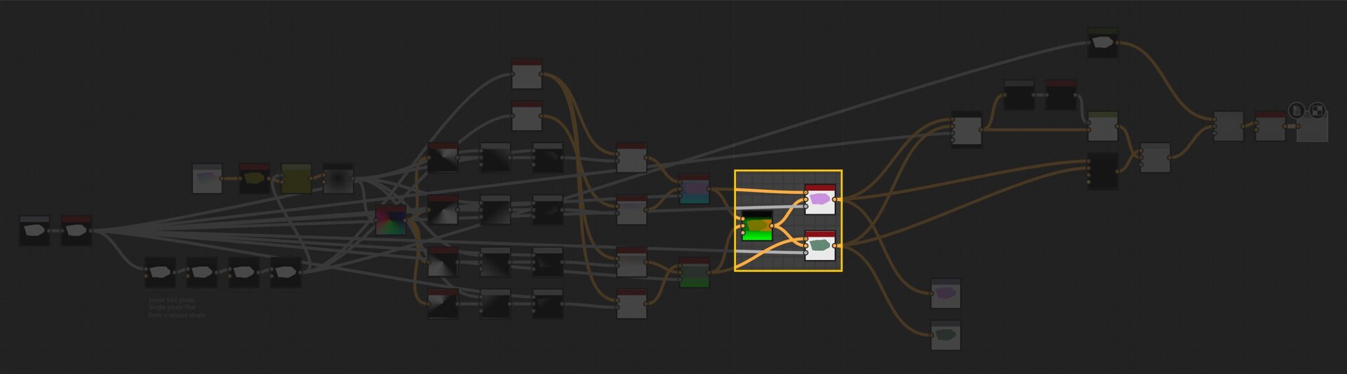
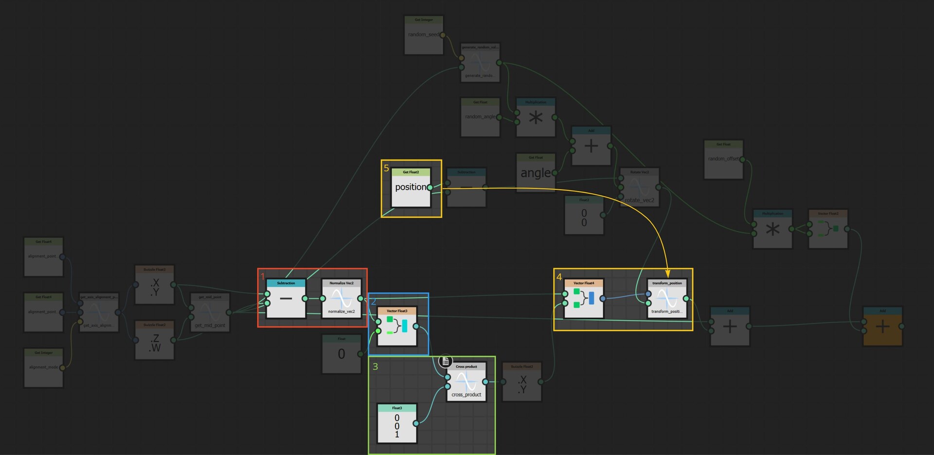
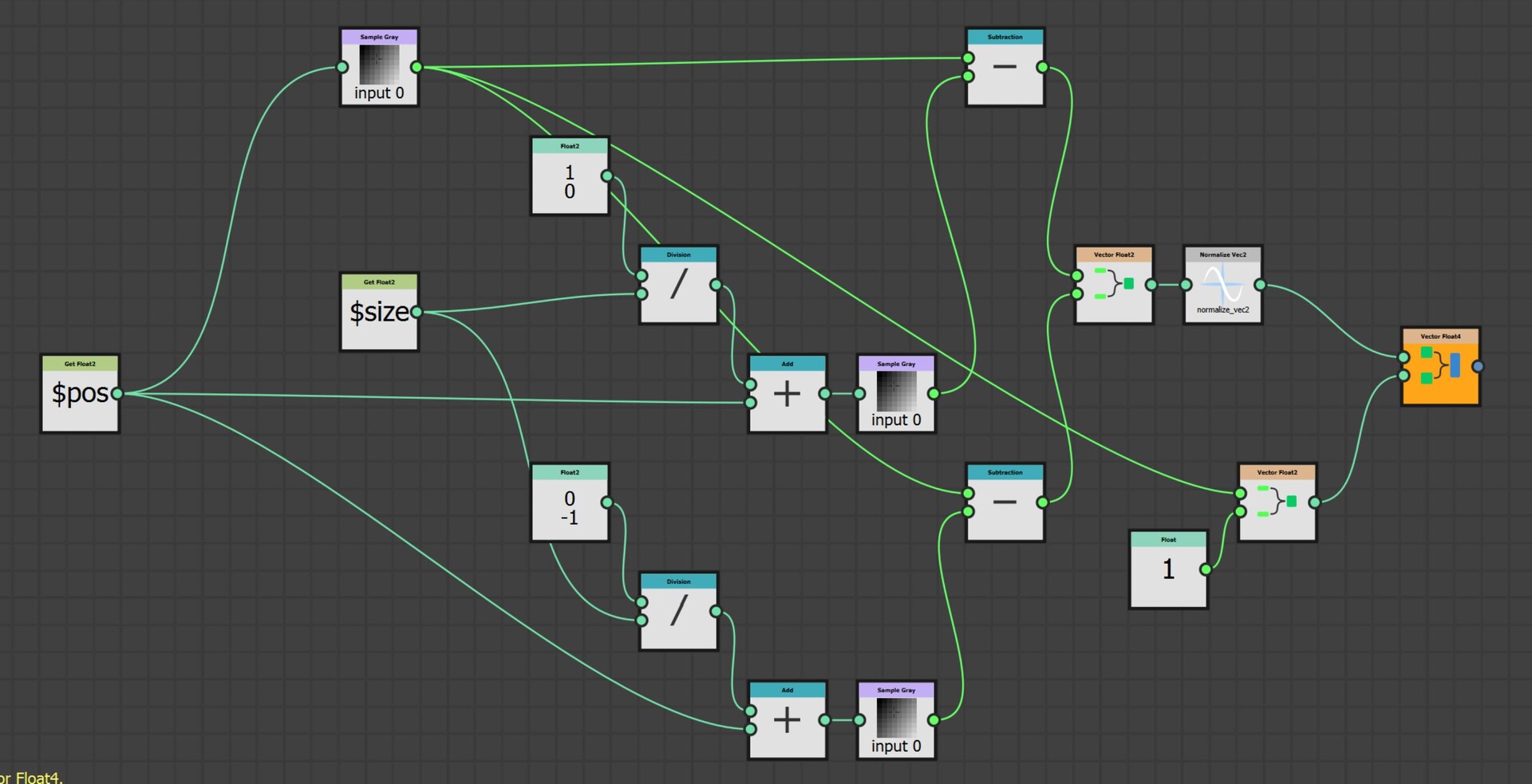
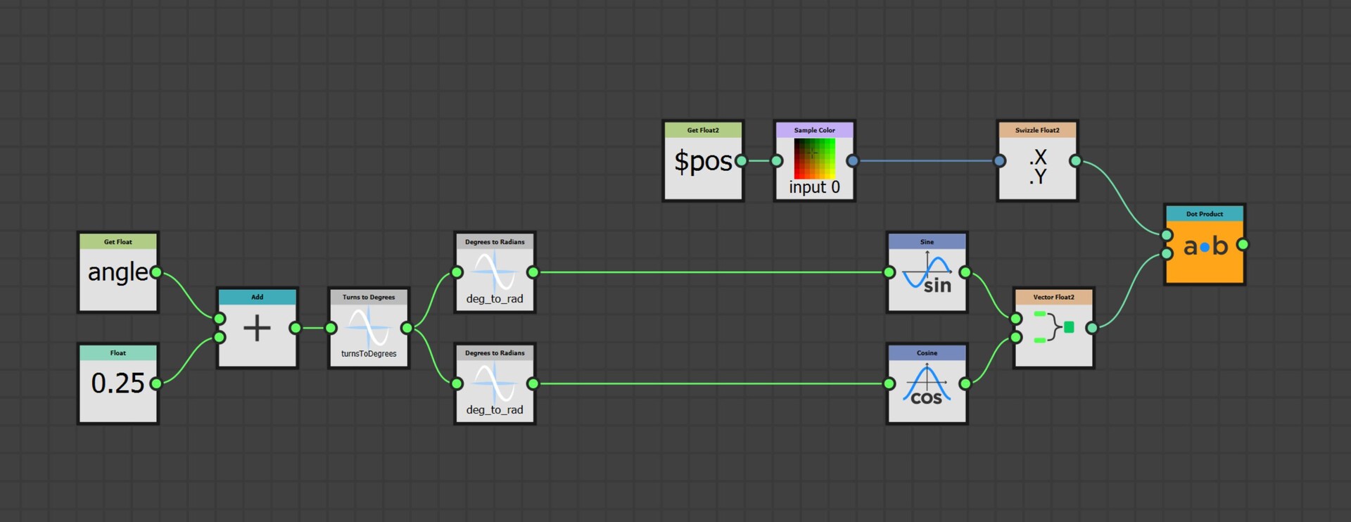
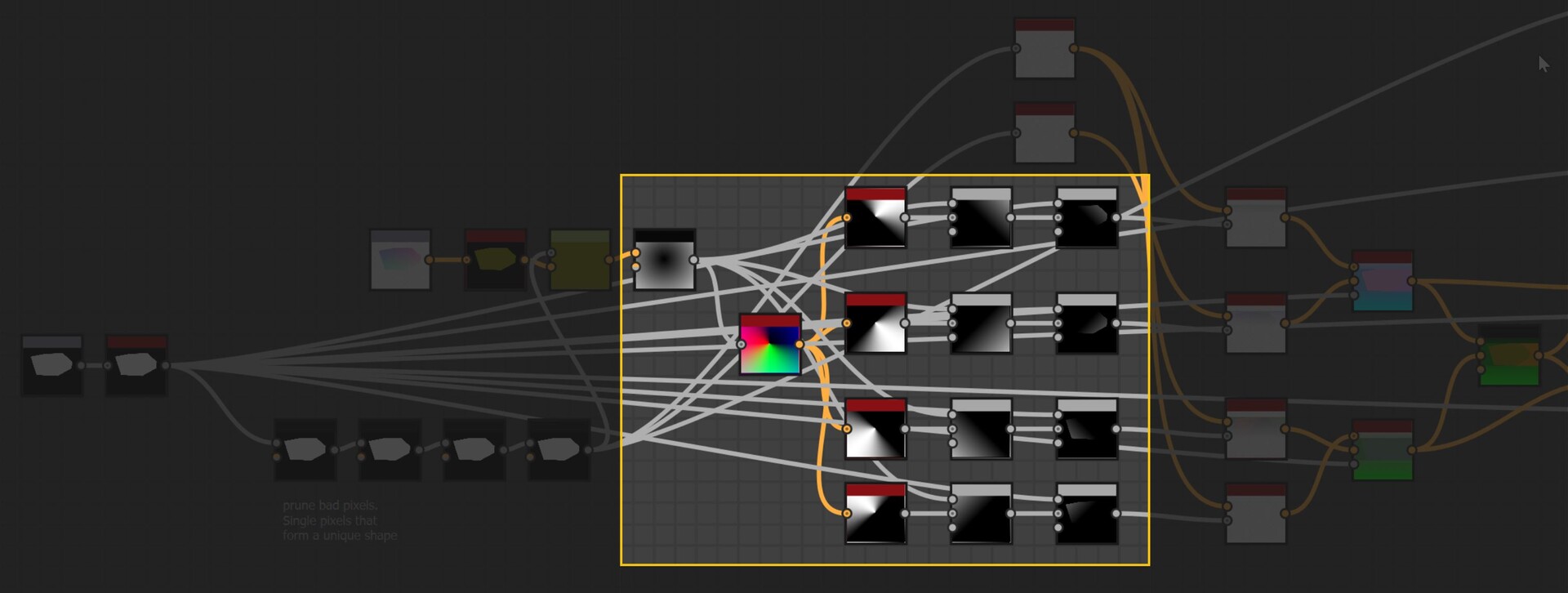
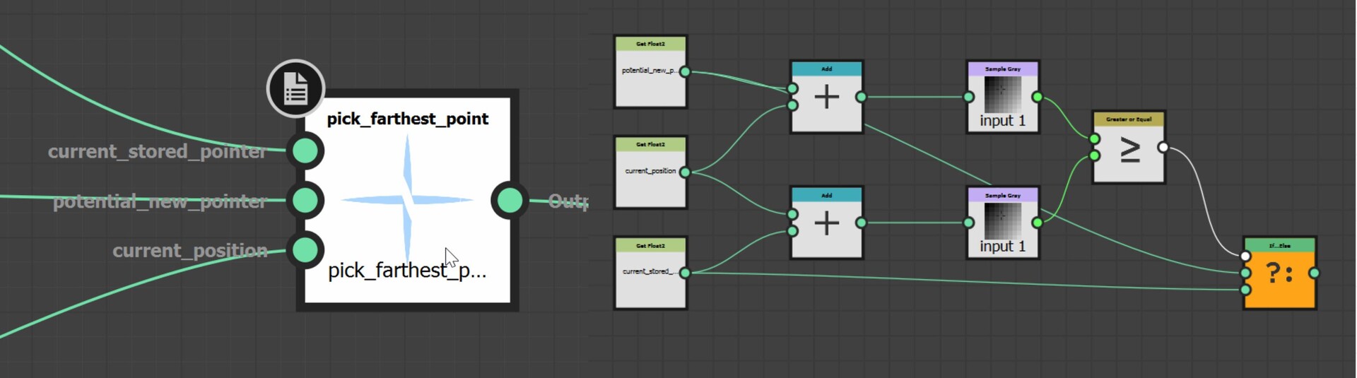
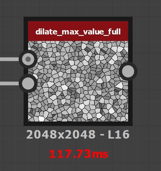
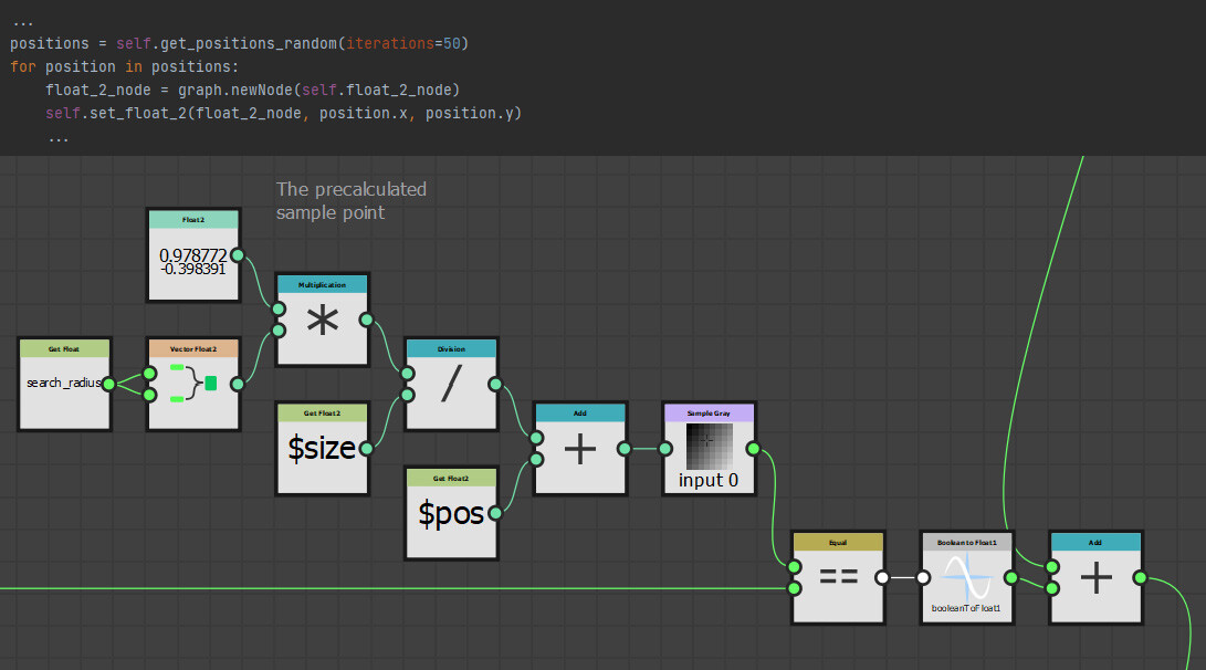
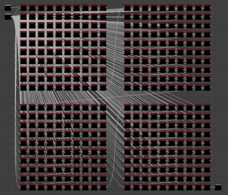
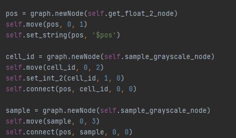
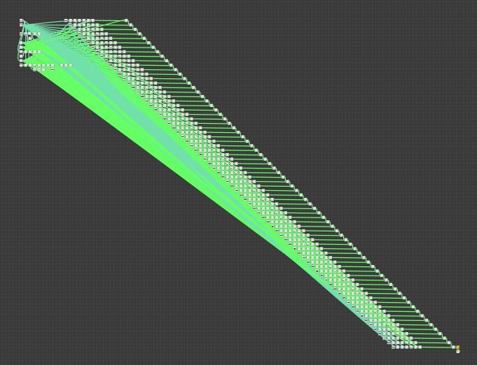
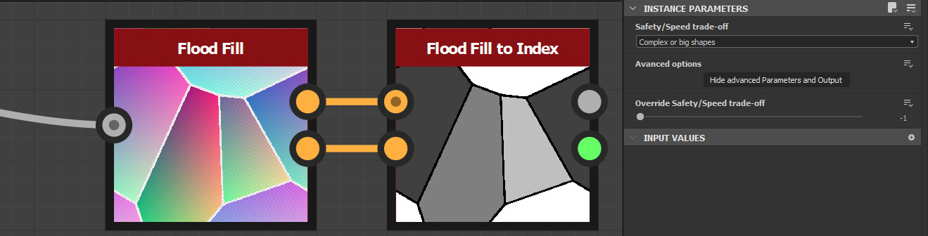
With our approach outlined, let's delve into the actual implementation. The core logic resides on the intensity parameter of a quadrant node in the FXMap, nested within the node structure.

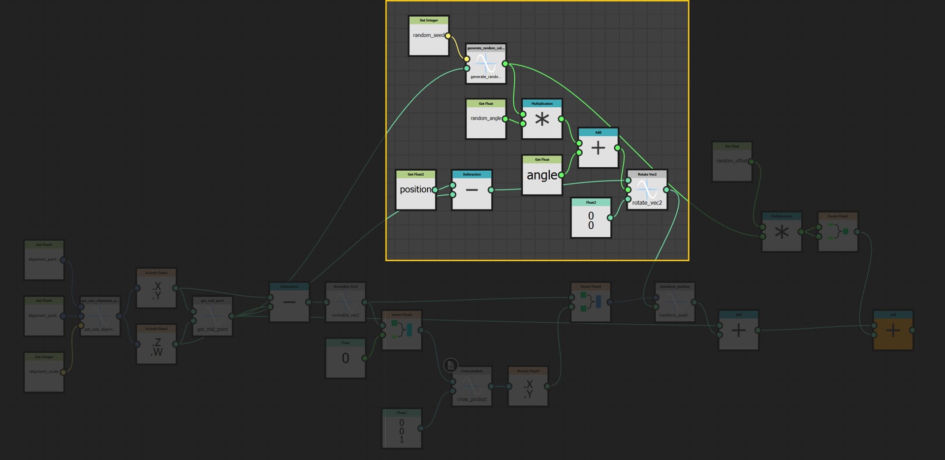
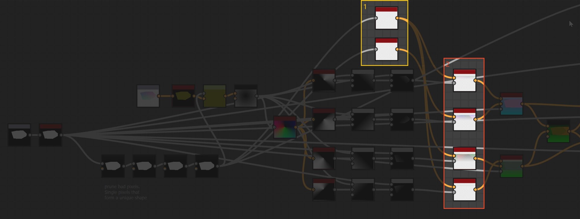
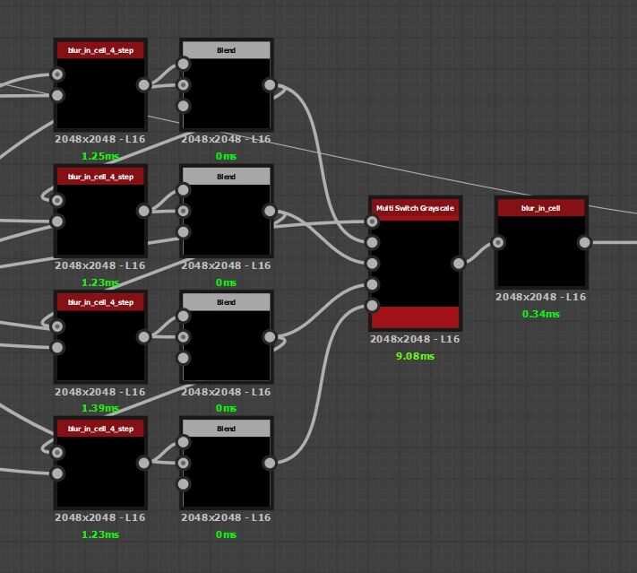
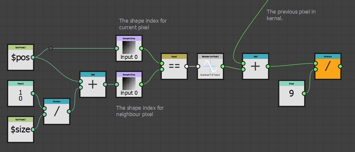
While there are additional nodes in the PDF graph, they relate to optimization and are not pivotal to our discussion. Our main focus will be on the function graph depicted below:

Binning

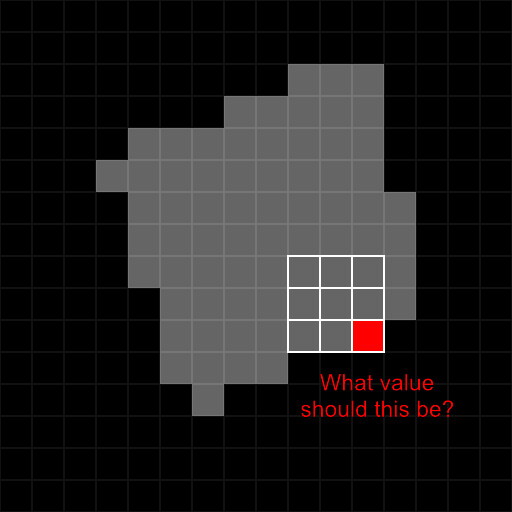
The first part of this function graph I want to talk about is value binning.

Our plan is to relocate every sample to its predefined location at the top of the image. To achieve this, we employ a process called 'binning', where each pixel value gets assigned to one of these 16 locations. Binning is accomplished through a method known as quantization. This process aligns each pixel value with a corresponding bin increment. We implement it as follows:

• First, for every sample, we get its intensity value using its position within the texture. This value will range between [0:1].
• We then multiply this intensity by 16 which is required for the next step to work.
• Next, we apply a flooring operation. This step effectively rounds down the result to the nearest whole number, aligning each pixel value with the nearest bin increment.
• Finally, we rescale the floored value back into the original range of [0:1]. This rescaling ensures that our quantized value stays within the original intensity range.

This quantization process effectively 'snaps' each pixel value to one of the 16 bin increments, which in turn will correspond to its new bin location along the horizonal. Think of this new value as an offset.

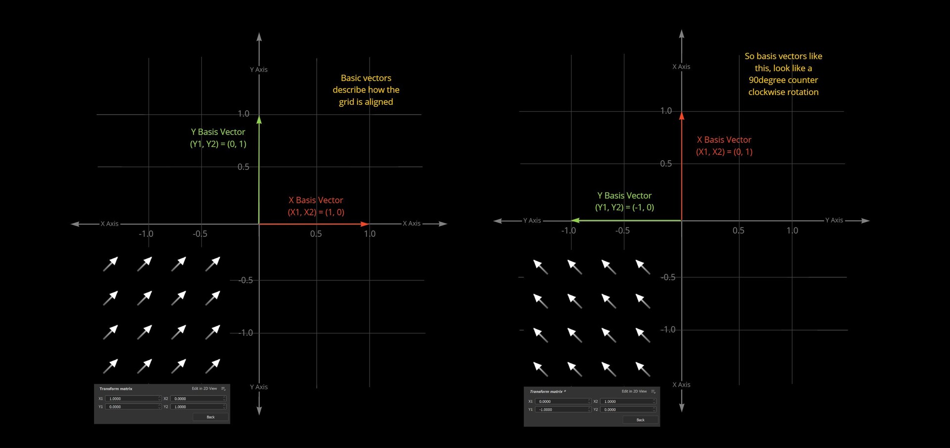
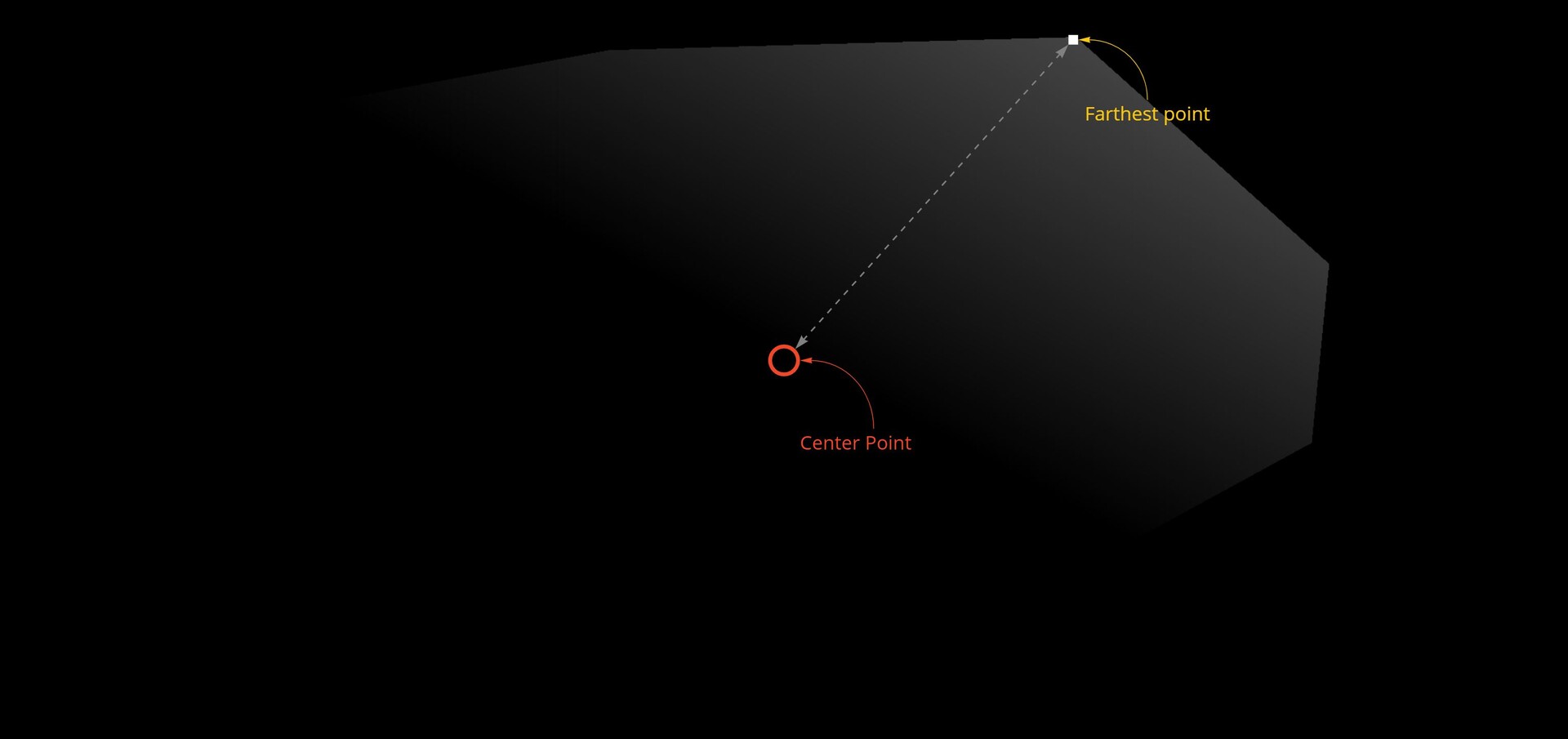
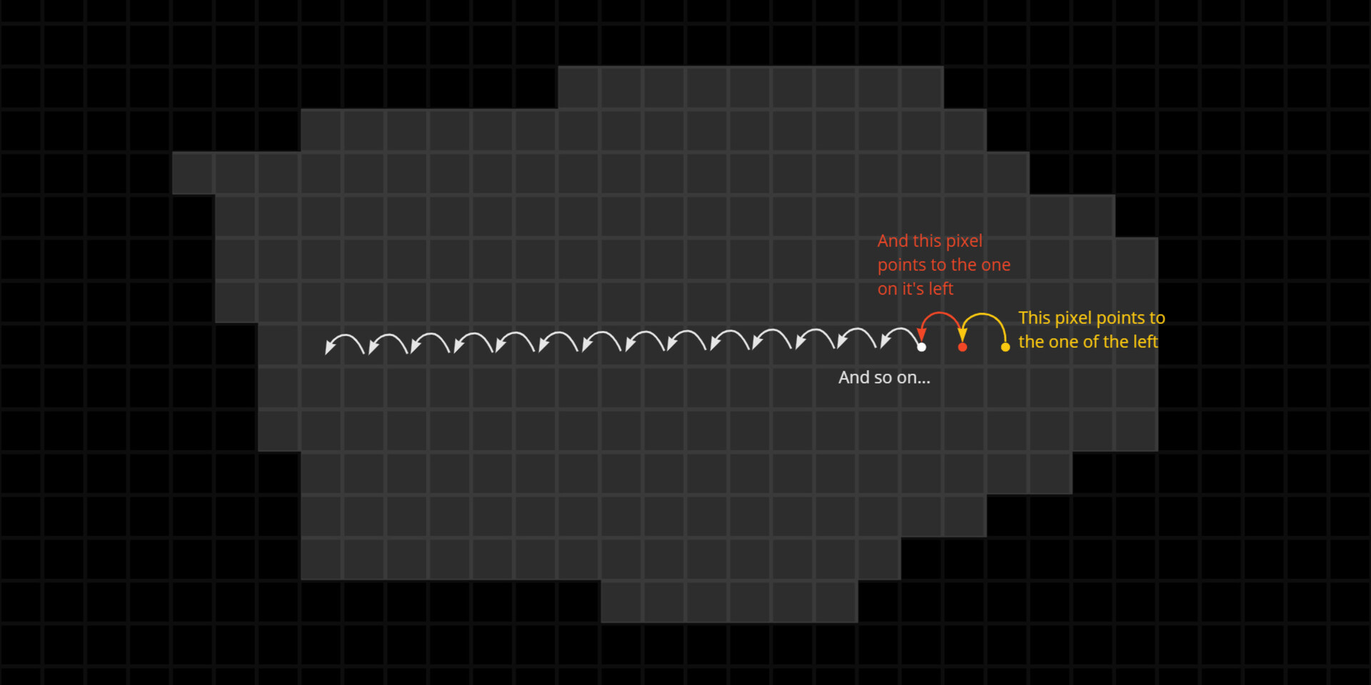
Repositioning

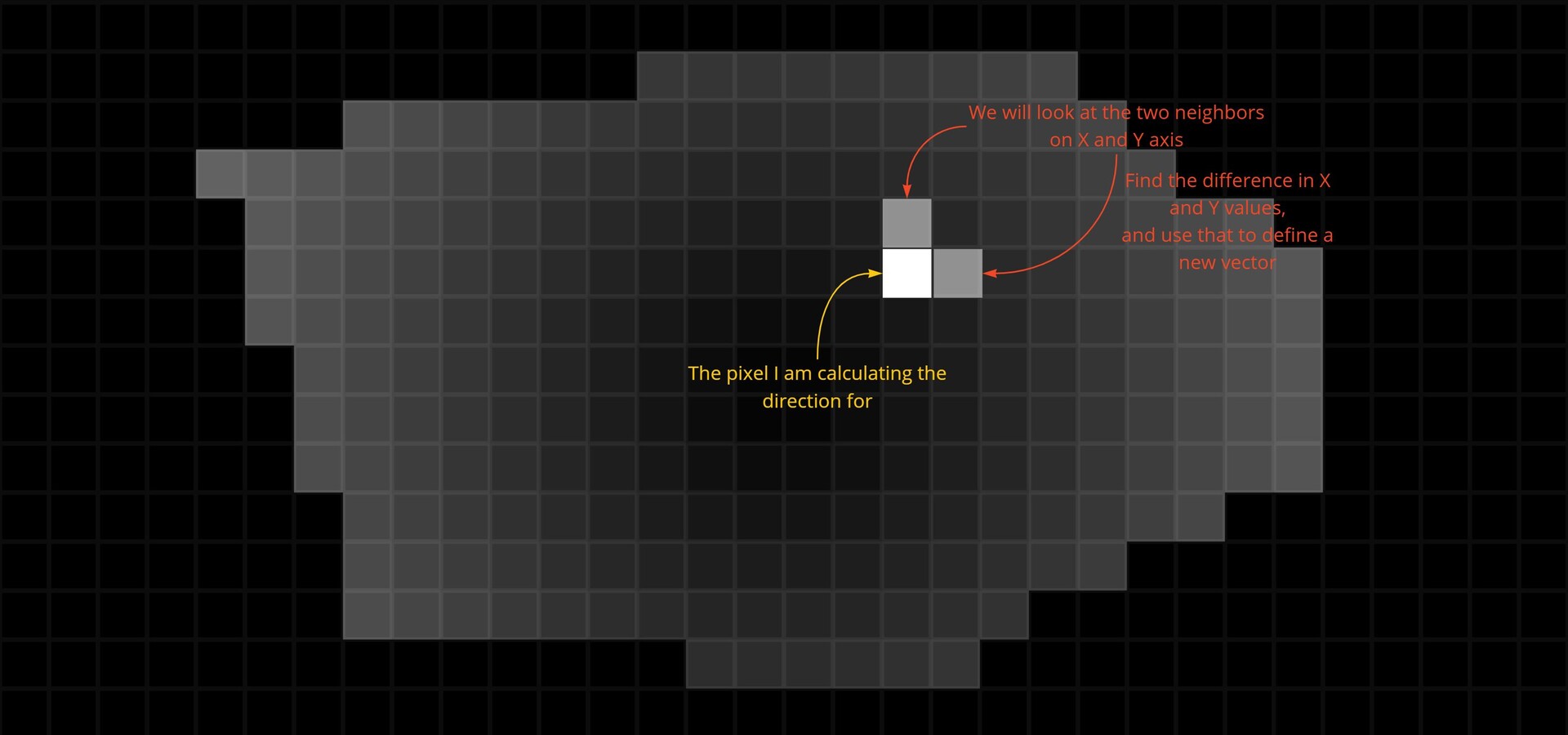
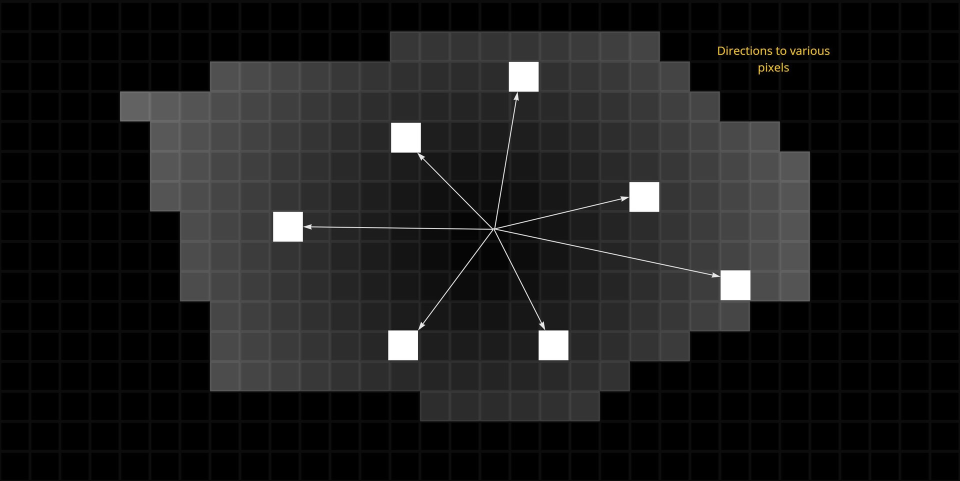
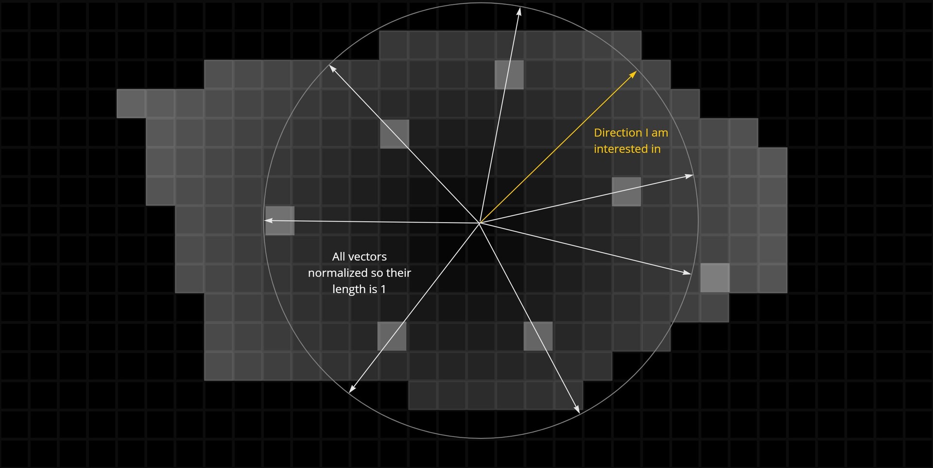
Moving the sample is done as follows:

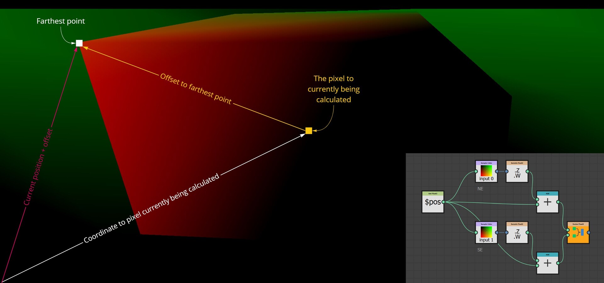
• Use the position variable to get the coordinates for each sample.
• Negate the coordinates to move the sample to the origin.
• Add the binned pixel value to offset it to the correct location.

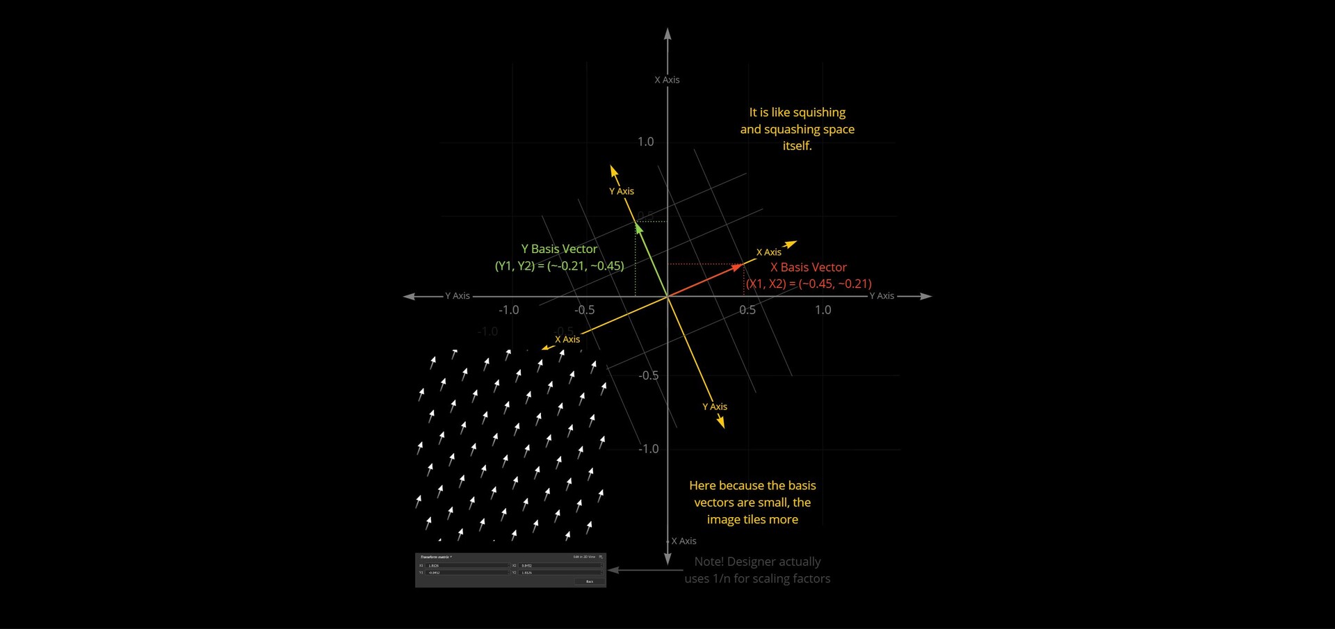
The negation process effectively resets each sample's position back to the image's origin point, which in Substance Designer is the top left corner (0,0), This is the reason why we are building the strip at the top. By subtracting the original position values from each sample, we align them all back to the origin. We then add the binned pixel value to each sample, offsetting it into its respective bin based on its intensity.

Counting

Once the samples are moved into their respective bins, they stack on top of one another. To count them, we could force each sample's pixel value to 1 (and set the FXMap node to add/sub). This configuration means that as samples of the same pixel value stack in each bin, their new value which we have set to 1 accumulates, effectively counting the number of samples in each bin. The stacked total at each bin then represents the count of samples for that bin's intensity range.

Normalization

Having determined the counts for each bin, we can now compute the final PDF. This involves normalizing the counts. We do this by dividing each bin's count by the total number of samples. In our example, since our sample grid was 16x16, the total is 256 samples. Dividing by the sample count gives us the probability of each bin. A small detail in this implementation is that this normalization is performed incrementally for each sample during the counting process, rather than as a separate step after all counts are tallied. This was done for simplicity sake but can happen during of after counting.

And thats it! We now have a strip of pixels who values represent the PDF of that image. All that remains is to crop out this little strip and there we go.

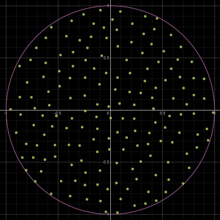
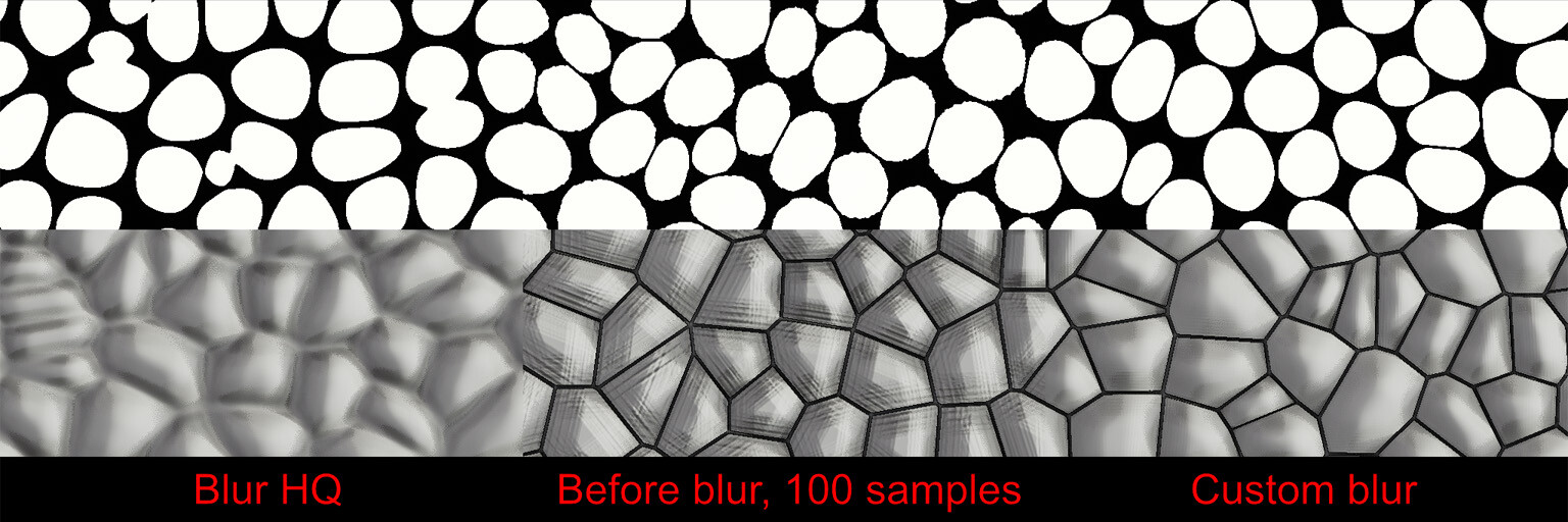
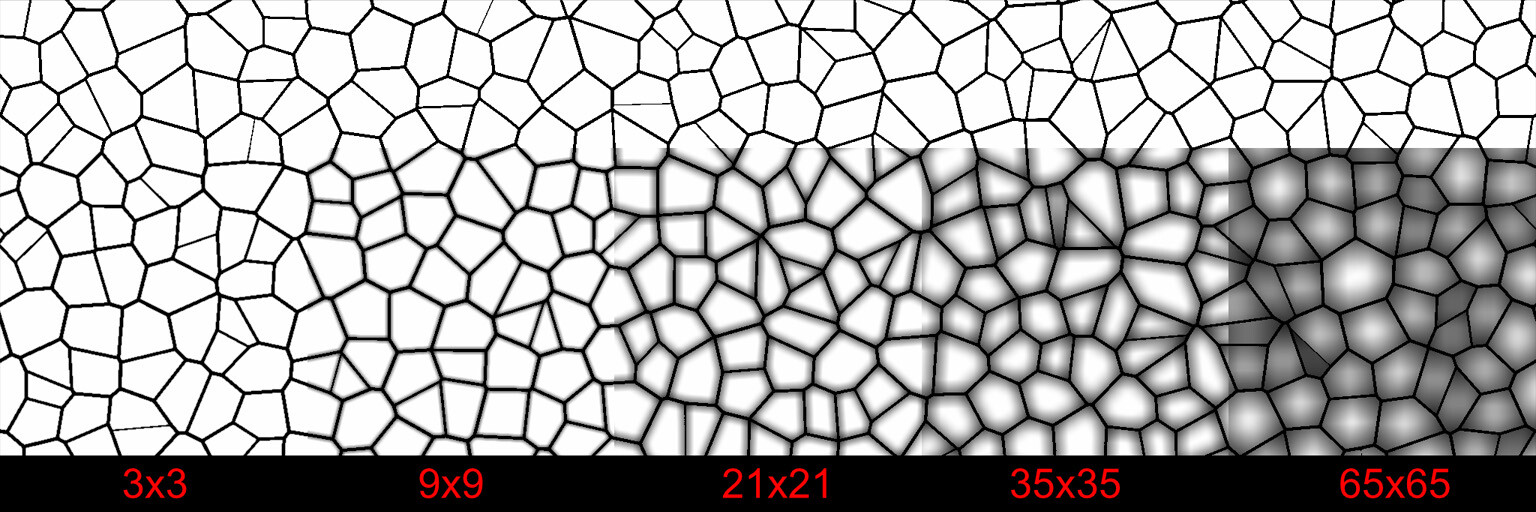
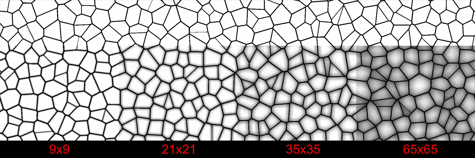
One key point to consider is the impact of sample resolution on PDF accuracy. A low sample count, like our 16x16 example, offers a very crude approximation of the texture's actual distribution, especially with high resolution such as 2048 or 4096 . In the actual implementation of the node, this process happens with 64, 128, 256 or 1024 bins, rather than just 16 but even with only 64 bins the accuracy is surprisingly good.

From my testing, increasing the bin count beyond 256 didn't offer much benefit in terms of accuracy, especially considering the additional computational cost. In fact, this method becomes impractically slow with anything beyond 1024 bins. Therefore, I found 256 bins to be an optimal balance between accuracy and performance and a good default value.

I hope this explanation has provided some understanding of the PDF computation and its practical implementation. Should you have any questions, thoughts, or feedback, feel free to reach out. The next part of this series will cover the CDF (Cumulative Distribution Function) calculation!

In precedent with my other Substance Nodes, this blog will accompany the Histogram Equalization and Specification nodes. It will be a three part series going through each node; how they work from underlying theory to Substance Designer implementation.

First we will discuss histogram equalization, then in part two, we will cover the Substance Designer implementation before moving onto the specification node.

If you don't know what it is, you can think of it as a kind of contrast adjustment for an image. Somewhat like doing an levels adjustment or using the existing histogram nodes in Designer.

However, equalization is actually something quite different. Here is a more formal definition: Histogram equalization is a technique used to redistribute the intensity values of an image so that they are uniformly spread across the available range (typically 0 to 255 for an 8-bit image). The goal is to make the histogram of the modified image as flat as possible, meaning that each intensity value is equally probable.

If any of that did not make sense to you don't worry, hopefully it will by the end of this post. So lets begin with understanding what a histogram is exactly and why we might want to equalize it.

A histogram is a graphical representation of the distribution of pixel values within a texture. The x-axis shows the range of pixel values, and the y-axis is a count of how many pixels had those values in the image. Visually, a histogram is often used to understand the characteristics of a texture, such as brightness or value range. Programmatically, a histogram is often used to analyze and adjust the contrast, brightness, and overall tonal balance of the image.

For our histogram below, these values are grouped into 20 evenly spaced 'bins' for easier viewing (but is it common to use 256). Then each pixel value which falls into a bin, is counted.

If you divide the histogram counts by the total number of pixels in the image (a process known as normalization) and draw a continuous curve through the points, this is called a Probability Density Function (PDF). The PDF tells you the probability of a pixel having a particular value.

While a histogram provides discrete counts, a PDF gives you a continuous probability curve, a subtle but important difference. In the context of everyday 3D art and textures, they can be used interchangeably, but it's important to understand the subtle differences between them since one speaks about counts and the other probability.

If you have spent any time with Substance Designer, you have likely seen the histogram. Typically we use nodes like histogram range or auto levels as a way to manipulate it, however unlike those nodes, which are linear operations (meaning your just moving the histogram up, down or stretching it), equalization completely redistributes the values in the image, changing the profile of the histogram itself. In the image below, notice how the linear operations maintain the bell shaped hump in the center, while the equalization changed the profile completely.

In the context of texturing, this can be incredibly helpful for all kinds of things. A common use case could be for generating color information with a gradient map or my color nodes (shameless plug). Equalizing the input image will ensure that you sample the full range of colors and not bias it to a small region of the color gradient.

If you cumulate the histogram, by going through each bin, summing the count from the bin before, you create what is called a Cumulative Distribution Function (CDF).

This function represents the probability that a pixel will have a value less than or equal to a given number. Unlike a Probability Density Function, which shows the probability of a pixel having a specific value, the CDF shows cumulative probabilities. It is not often you will come across a CDF in day to day texture work, but in the context of image processing, this information can be very useful and as you may have guessed, it is crucial for performing histogram equalization.

Lets look at some histograms to familiarize ourselves with how both PDF and CDF looks for difference types of images.

In the image below, we have a relatively mid tone image where most of the pixels are floating around the mid range. Notice how you can see this behavior represented both in the PDF with its hump in the center and the CDF transitioning sharply in the same location.

In the next image, the values are mostly residing in the upper range, which moves everything up in the PDF and CDF also.

While a darker image pushes everything to the lower range.

One very important PDF/CDF is that of an image where every pixel is equally likely. Such as a linear gradient.

Notice here that each histogram bin has exactly the same count, thus each pixel value has the same probability of occurring, which in turn means the CDF is a perfectly straight line. Why this is the case is essential to understanding equalization, so take a moment to think on it if it feels ambiguous. Here the CDF is saying that each pixel value (x axis) has the same cumulative probability (y axis). Or, put in other words, by half way through the value range (x axis), I will have seen exactly 50% of the values (y axis). Or, by value 0.75, I will have seen exactly 75% of the values and so on.

Histogram equalization works by remapping the image pixel values according to its CDF. What that means in practice is computing a CDF for the image then replacing each pixel value with the corresponding CDF value.

If you were like me, this seemed incredibly simple, but also...what?! Sure, remapping pixel values is straightforward (gradient dynamic node in Substance), take one value and convert it to another based on that function, but it was not at all clear to me why remapping with the CDF would work, much less one generated from the image itself.

To better understand this, consider the transformation as a function, let's call it f(x). In this equation, x is the input image, and the output we want to be the remapped equalized image. It's logical to assume that f(x) would be related to probabilities, after all we are trying to equalize the image and the CDF does indeed provide a probability distribution for the image. But still, it wasn't clear to me why this works. I did not have an intuition or clear visualization of what was happening.

Recall, the CDF tells you the probability that a randomly picked pixel will have a certain intensity value or lower.

When remapping, I like to visualize it as projecting that CDF curve onto the x=y line. This line also happens to be what a perfectly equalized image CDF looks like, as we saw before.

This projection is essentially saying something like "we want 80% of the pixels to have occurred by value 0.8, not 0.27 which is where it was before". This is why using the CDF works, its taking all the probability information in the image, and forcing it to be linear.

That's all there is to it really. It is a single remapping from one set of values to another but all the mystery and magic comes from those set of numbers containing information about the pixel value probabilities.

And that concludes the first part of our jump into histogram equalization, I hope it was useful. In the next part of this series, we will go through how this can be implemented in Substance Designer.

In the last part we just finished off creating our step function and now we will be implementing the rest of the node. The output of the step functions are images with pointers to the farthest pixel in a given direction.

This is in fact everything we need to calculate alignment points. For every pixel, we can now find relevant corner points and form a transformation matrix from it. 

The first step however was to convert this information into uv positions, much the same as the flood fill to position node. This is done by adding the current pixel position to the pointer vector. 

So now I have two maps which output uv position of the four corresponding points in R,G and B,A respectively.

There is a setup here that dilates these uv position through the shape by sampling the position at the center of each shape. However, I will gloss over this since its not actually needed and not important for this blog. I added it before figuring out the counter clockwise issue! I left it in the source file though, should you be interested in taking a look. 

With these four points, it is then possible to align an axis grid by taking the mid points between 2 of them. I ended up exposing a variety of different alignment modes, which essentially came down to picking which two points to align an axis too.

And here is an image showing the alignment points applied to a real example. 

Now we have 2 points to form an alignment transformation matrix from, lets look at how that actually happens. For this we need to understand how transformation matrices work. More specifically, a 2D transformation matrix. The one you find on the transform 2d node.

In the transform 2d node, the values for X and Y correspond to the coordinates of two vectors which will define a grid. These are called basis vectors.

So, X1, X2 are the x, y components defining what the X basis vector should look like. Y1, Y2 the x, y components of the Y basis vector. These describe what the X and Y  lines of a new grid should look like. You can think about it like rotating, squishing and squashing space itself into this new grid defined by these basis vectors.

Because we have two alignment points, we already have what we need to calculate at least one of the axis! We can use the delta between the two alignment points as an X  basis vector. 

But what about the Y axis? For that we can use a cross product. The cross product will give you the vector perpendicular to two input vectors in 3d space. 

So, if we were to assume our texture is in 3d space, where the X axis is already known and the Z Axis looks directly towards the view, then the cross product between those two vectors would give us Y. 

And here is the implementation for that. (1) We first construct the X axis and normalize it so the vectors length is 1. (2) Then convert that to a 3d vector by appending a z axis. We set the z component to 0 because we actually want this vector to rest on the texture plane. (3) Then cross product with a vector that points along the Z axis, which gives us the Y. (4) Since X and Y now both rest on the texture plane, we no longer need the z component, so that is removed and both vectors stored as the basis vectors of a 4x4 matrix. (5) Finally, the uv positions are multiplied by this matrix to perform the actual alignment. 

Also to note, there is a whole section here dealing with rotating the uv coordinates before being aligned and this was to provide some angle parameters to the user. I will leave you to explore that on your own too =)

However, as a small gotcha, if you are trying to implement this yourself; While Designer does come with a transform position node, it makes some assumptions about your uvs, so I needed to reimplement my own version to do the matrix multiplication.

And that was the last piece of the puzzle. When we input an image, it will align the uvs to each shape. Here is an image showing an example.

So this concludes everything I wanted to discuss about the node implementation, but before we close out I did want to briefly talk about why all this doesn't really work!

Firstly, there is the limitation of convex shapes. We alluded to this before; the fact I am using the bounding box center to determine the distance means some shapes will fail to find a valid point.

While this might not be a deal breaker (after all the use case is for convex stones), it does mean the setup is not 100% robust.

The biggest and main problem however is simple, this method is unable to find appropriate alignment points for a lot of shapes. This stems from the bad assumption that corners are going to be in the 45 degree directions (or which ever you pick) and the farthest point might not necessarily be in a good corner either. The node is particularly sensitive to shapes that are on the 45 degree angles.

In the field of computer vision, there is an image processing concept called image moments and this is used to calculate things like weight, centroid and shape orientation. The second order moment specifically is used to find the orientation and can be thought of as finding the axis of minimum energy required to spin the shape. This I think would be a much more robust way of approaching the problem!

I recommend watching this wonderful lecture on the topic here https://youtu.be/ZPQiKXqHYrM

For now though, I am done with this problem and may pick it up again in the future. I will be putting the source files on my store (free) should you want to dig into the node further, Even though this didn't pan out as I wanted, I do hope it was interesting to you none the less.

Before closing out, I would like to specifically thank Igor Elovikov https://www.artstation.com/elovikov who was the one who really reverse engineered the flood fill node and was kind enough to share his findings with me. I definitely wouldn't have figured it out on my own! And of course Stan Brown https://www.artstation.com/stanbrown who is the one who got me hooked onto the topic and letting me use his textures for testing!

If you would like to take a look at the source files, they are available on my store https://www.artstation.com/a/14364831

Thanks for reading!

So where were we? To give a little recap, we needed to calculate the distance from the center to any pixel so that as we are stepping around the shape edges, we can use that value to find an appropriate corner point.

The issue right now is we can only deduce the farthest point, not the farthest point in a particular direction. We need a way to calculate that too.

My idea to solve this was to calculate a direction map and then compare a desired direction against that texture. This could then be used to modify the distance map. 

Lets look at how that works. It is possible to calculate the direction a gradient is sloping by finding the delta between neighbouring pixels. The delta is the name given to describe the change in a value between two points. So, if we plot a line on a graph. We could pick any two points on that line and say the delta in x (the change in x value) between those two points is the difference between the x value of point 2 and point 1. The same for Y axis.

So we could look at two pixels, in x and y respectively and use the values from the distance map to calculate the delta. 

Which, if the then plot on a new graph, and draw a line from the origin to the point, it will give us the direction we need. The vector dx, dy is the direction the distance map is sloping. 

So doing this for all pixels, we would end up with a texture which describes the direction of the gradient at every point in the shape.

Then in order to compare the vectors with a chosen direction, we must normalize the result, so every vector now has a length of 1. 

Taking the dot product is then comparing how close every direction is to the chosen one. Where the vectors are pointing in the same direction, the output is 1. As they become perpendicular, the output approachs 0 and where they point in the opposite direction, it approachs -1. 

Here is the implementation for that. It is split across two pixel processor nodes. 

Now I can multiply my distance map by this directional map and use that to find the farthest point in the step function instead. 

This is done four times in four directions. 

Now lets look at the step function. We already saw how this works for the flood fill node in part 1, and this will be almost identical. We will store pointers to neighbouring pixels until finding an edge, then start spinning around it.

The only difference is, instead of storing the vector to a reference pixel, we will store the vector to the farthest pixel. This is as simple as storing the one with the largest distance value, taken from map we just calculated. 

So, looking at an overview, we have some initial setup of values (the first pass in the step function), then successive jumps with each jump updating its pointer to a new farthest pixel. 

And here are the passes of successive jumps. In my testing I found 8 passes to be to little to resolve fully and 16 to be just fine. However, I added more steps just in case and setup some switches on blend nodes to toggle between if needed. 

You may notice too that I have 2 nodes for the initial setup of values, with one going into 3 step functions and the other only into 1. 

The reason for this was because in that particular direction, the values were not converging correctly on some shapes. Notice how on this shape there is a gap in the right hand corner.

To be honest, it is still unclear to me why this is happening, but I did notice it was only occurring when calculating the direction to the bottom right. This lead me to suspect it was something to with stepping around the edges in a clock wise pattern. So this second node is stepping counter clockwise instead. Indeed it fixes the issue, but if anyone has insight into why exactly we must step counter clockwise when calculating the bottom right direction, please let me know!

For now we will end part 3 and return in the next post to see what the step function outputs and how it was used.
https://www.artstation.com/blogs/benwilson/nZ67/alignment-node-development-part-4

In the last part we looked at the flood fill node and how it works. In this part, we will see how this applies to the alignment node and start discussing the details.

The goal is to find some points which can be used to form an alignment matrix. So, the idea I had was to more or less do the same thing as the flood fill. Step around the edges, asking if this reference pixel is a 'corner' or not. Ideally, we would end up with an output that looks something like this.

The first idea I had was to use an if statement very similar to the one in the flood fill, where it finds a reference pixel; Is the pixel farther up and right? Is the pixel farther down and left? and so on...

However, this turned out to not work well. Sometimes the node would never converge to a single pixel. I think this is because my if statement was setup with an AND condition: If farther AND farther right. Take this pixel for example, it would fail because while its reference pixel might well be farther to the right, its not farther right and farther up. Essentially I was finding local minimums and never converging fully.

You might think that you could stagger the if statement instead. Something like: If farther right, then check if its farther up. The issue here however is you end up biasing the result to a particular axis. 

I tried a variety of these condition and never found one that worked. In the case of flood fill, I think it works because its only interested in finding one pixel and it doesn't matter where exactly. So they are able to construct an if statement which is defined fully. In this case though, we need a particular corner, in a particular direction, and that is harder to define.

So instead I decided to use the distance from the center as a way of weighting the question. The idea is this: Always pick the pixel which is farther away from the center, but only if it is pointing in a particular direction.

Now, before we discuss how that is implemented, there is an interesting question. What is the center of the shape? The centroid may be the obvious one, but we don't immediately have that information. And in fact, to calculate that we would need to use a concept called image moments. We will talk more about this at the end of the series. 

The next logical one might be the center of the bounding box. We do in fact have that information to hand already, it comes with the flood fill node. However, both of these come with other problems; its possible the center actually lays outside of the shape.

Another approach may be to take the center of a best fit circle. This is something I covered in my last blog series https://www.artstation.com/blogs/benwilson/2WpV/flood-fill-to-corners-development-part-3

The issue here is that its quite a bit more expensive to compute and may not be very 'center' in some shapes.

In the end, I decided to use the bounding box center for simplicity. I wanted to get the node up and running quickly to see if it would even work anyway. After all, my use case was a typical convex shape anyway.

So lets look at how to calculate the distance from the center. There are 3 steps I took for this:

1. The first is to dilate the flood fill to position output, which if you didn't know, gives you the uv position of the bounding box center for each shape.

2. The second is a pre pass to try and prune floating pixels which were causing issues in the step functions. Here you can see how the pre pass identify and remove floating pixels.

This is done by looking at each neighbour pixel, counting them up and outputting black if the pixel is isolated. So if a pixel is surrounded by black, except for one pixel, then I assume it to be associated with a shape, but isolated.

There are 4 passes to this, because pruning one pixel might produce another isolated one (in the case of a line), reasoning that four will probably be enough. This is quite hacky, but I want to emphasis again that I am not worrying about making the node fail safe and robust at this point. I needed to prove the theory would work first, which as it turns out, didn't =)

3. This last part is very simple, take the distance between the center point and the center pixel. The farther we are from the center, the larger the distance value will be.

However, this introduces an interesting error when applied to the full tiling texture. When we are close to the border, the center point might actually be on the other end of the texture, leading to artificially large distance values. 

To solve this, we must offset the texture by one full tile and then compute the distance, taking which ever is the smallest. Do this for all 8 directions and it will fix the tiling. 

This wraps up part 2, in part 3 https://www.artstation.com/blogs/benwilson/opoN/alignment-node-development-part-3 we will continue directly from here and discuss how to use this newly computed distance map. See you soon. 

Hi all, I am back with another blog series on a Substance Designer node I was recently working on.

It is designed to align an input image to flood fill shape orientations automatically and this series will be a deep dive into the workings of it.

This series will be a little different to the last one in that this node is actually a failure in many ways. Ultimately, I did not deliver on the goal I set out to reach but since I learnt a lot and think there is some interesting topics here, I wanted to do a series on it none the less.

While I do not recommend using the node, I have uploaded the source files to my store, so you can do so if you wish. https://www.artstation.com/a/14364831

We will start with setting up the problem, defining what exactly we are trying to solve. Then talk briefly about how I planned to approach the problem. After that we will dive into the flood fill node and discuss the algorithm and how its implemented. From here we can see how it relates to the implementation of this alignment node by looking at the math and node setup for everything. Finally, we will close out by discussing where the node falls short and why, and propose a potential better solution.

I will be assuming you have read my previous blog or have some familiarity with the pixel processor node for this, so make sure to skim through that if you haven't already! https://www.artstation.com/blogs/benwilson/PlRE/flood-fill-to-corners-development-part-1

SETUP THE PROBLEM

Let us begin with describing what problem I was trying to solve. I wanted to solve automatically rotating textures to individual stone shape orientations, given its input mask.

The use case I had in mind was texturing organic stone walls with very directional material information.

The general idea I took, and the one we will go through in this series, was to find corner points in the shapes and use those to align the uvs.

As I mentioned before, I do not think this is necessarily the best approach, but we will talk more about that at the end of the series.

FLOOD FILL NODE

The best place to start is with understanding how the flood fill node works. Firstly because it really underpins the whole approach I took, but also because it's just interesting.

Flood fill works in a very similar way to a jump flood algorithm. If you are unfamiliar with it, I highly recommend reading up a little. This blog by Ryan Kaplan is great https://www.rykap.com/graphics/skew/2016/02/25/voronoi-diagrams/

I also mention it in my last blog post about the corner node, where I unintentionally implemented a crude version of it. https://www.artstation.com/blogs/benwilson/2WpV/flood-fill-to-corners-development-part-3

There are two key points which are relevant to understand about the jump flood algorithm.

1. You can query and store any data, not just distance to center. If you can define your query fully, you can flood it through a texture.
2. There is no reason step increments must be in a grid pattern. You can step in any direction or shape you want, and we will see this later.

If any of that didn't make sense to you, then it's ok. Hopefully the visualisations going forward will make everything clearer.

If you are reading this, you are likely already familiar with what the flood fill node does. However, lets define it here on a more low level. The flood fill attempts to to find all edges of shapes in a binary image and calculate useful information like bounding box, uvs and how many shapes there are. It does this by finding a 'reference' pixel per shape, so it can guarantee that for every shape in the image, there exists only one corresponding pixel. This is how the flood fill to index node is able to count the number of shapes. And it does that by finding and spinning around the edges, gathering data about the shape as it goes.

This edge spinning is implemented as a series of increasing steps or jumps, which is the analogy to the jump flood algorithm. So lets look at that; the edge spinning is broken down into passes.

In the first pass, it will output a 'pointer' map. This is a texture where every pixel is pointing to its immediate neighbour to the left. When I say pointing too, I actually mean its storing the vector to that neighbour pixel from its current position in uv space. Or another way of saying it how many pixels do I need to move from where I am to reach that new pixel.

This vector is stored in the Red and Green channel. 

However, rather than blindly storing the left neighbour, there is some logic to determine if the pixel is on an edge. If it is, it will store the next clockwise pixel along that edge instead. 

So after the first pass, we have a texture containing pointers at every pixel that looks something like this. 

In the next step, it will look at the pointed pixel, find out where that one is pointing, then update itself with the same logic. 

And this process repeats in all subsequent steps, each time making larger and larger jumps.

This is what gives rise to the spinning behaviour. Each pass makes incrementally larger jumps and when it finds an edge, it starts spinning around it. Now, as it makes each step, it also queries something about the pixels. In the case of finding a reference pixel, along with storing the pointed pixel, it also tracks the location of a reference pixel. At each step, it asks:

Is the pointed pixel's reference pixel farther up in Y and if so, farther right in X than my current reference pixel? If yes, it will update the reference pixel to this new one, otherwise it will keep it's current reference pixel. This reference pixel is stored in the Blue and Alpha components.

After enough passes, every pixel will have looked at another that was either updated directly or saw another pixel that saw another pixel who was updated. Quite the brain teaser, but essentially this is the same concept as jump flooding, except constrained to a shapes bounding edges. At the end of the passes, the comparison result 'spreads' through the shapes in the image. The net result of this is a texture where every pixel points to some reference pixel, the top right one in this case. 

And to clarify, this vector is stored in the Blue and Alpha component. Red and Green will still be pointing to some arbitrary location on the edge after all the passes.

The flood fill node does a lot of other things too. It calculates bounding box information during these steps, it identifies inside and outside edges and there is a whole part of the network dedicated to solving shapes with holes. I am glossing over a lot of details too, some of which I have not fully understood myself, but what we just went through is the gist of it, and what you need to know to understand how this alignment node works.

In part 2 https://www.artstation.com/blogs/benwilson/AmVz/alignment-node-development-part-2, we will begin looking at the implementation for the alignment node itself.

Hi all,

I am happy to announce that I joined Epic Games Quixel as a Tech Artist. As such, I am releasing my Designer Plugin BWTools open source, along with a new update. I have put considerable effort into these tools, so am very happy they are now more accessible to folk.

So what's new in this version? The most notable change is a new plugin, BW Framer, designed to help with adjusting your frames and some improvements to the existing layout tools. There is also new documentation on a dedicated site and not tucked away in my artstation blog. Please take a look through if you plan to use the new version. Aside from this, the whole toolset have been rewritten to make the code cleaner for this open source release. If your interesting in learning Designer's API, check out the code on my GitHub.

Here's a more detailed breakdown of the changes and a link to the download

https://www.artstation.com/a/848543

General changes

• Replaced the top toolbar icon with a menu bar to access the tools. It now lives next to the Help menu.
• Moved all graph related tools to the graph view toolbar, which can be toggled on and off.
• It is no longer possible to run the tools on graph types currently unsupported by the Designer API. This was previously causing a crash with the latest release.
• Added more detailed tooltips.

New plugin BW Framer

Reframe a selection of nodes quickly and provide default settings for the frame. No more manually adjusting frames after moving your nodes.

BW Layout Tool Changes

• Considerable performance increase when running the layout tool. On average a 66x increase in performance. (102 seconds down to 1.6 seconds to run the tool on my test graph)
• The mainline feature (which pushed nodes back) is now toggleable.
• Added multiple layout styles.
• Added a snap to grid option
• Added option to run BW Straighten Connection after running the layout.
• Several bug fixes in layout behavior (the default behavior may be a little different in this release).

BW Optimize Changes

• Removed features which are now natively handled by Designer.
• Fixed a bug which would incorrectly identify some nodes as duplicates.

BW Straighten Connection Changes

• Now supports two different layout styles.

BW PBR Reference Changes

• Is now opened from the new menu bar.
• Removed custom color support in order to simplify the code for this release. The feature was barely used.

I want to thank everyone who had purchased the tools, your support is very much appreciated and if you purchased the tools in the last month, please dm me.

Welcome to part 3 of my development blog! This is a continuation of the last two posts, so make sure to read them if you haven't yet!
Part 1
Part 2

In the last post we discussed using a circular kernel and explored different sampling patterns. We had moved away from using a stride value and instead defined a maximum search radius and scaled the sample points with that. However, textures with large variation in shape size will have problems as the search radius increases. In fact, we loose smaller shapes entirely, due to the radius becoming larger than the shape itself.

So what if we could scale this radius value per shape? In case you are not aware, the flood fill to bounding box size actually outputs a normalized size for each shape. Exactly what we need.

The values in the map are normalized to uv space, meaning if we multiply them by the texture size, they will actually give us the bounding box size of each shape in pixels! 

If we were to then scale the search radius by this bounding box size, our kernel would then respect each shape individually.

Of course, the bounding box size is going to be different for the x and y axis, so lets take the largest number of the two, max(x, y),  as a start. This is also the default on the flood fill to bounding box node. 

Left is without dynamic scaling, right is with. 

A big improvement already! However, a lot of the shapes are still becoming very small or disappearing again. This is due to the bounding box not accurately representing the shape in question.

Diagonal thin shapes being the worst offenders. Notice how poorly the box fits around the shape.

The flood fill to bounding box node has two other outputs, the values for x and y values respectively. Maybe we can get a more accurate bounding box by averaging the two, rather than taking the max. The image below shows a comparison between max(x, y) and (x + y) / 2. Green denoting how much we have improved.

Another good step forward but we are not quite there yet. Some shapes are still disappearing. After consulting with my lead again, he suggested I look into calculating the largest circle that fits inside the shape. In fact, the distance node can be used to generate this value. If we set a value of 256 on the distance node, it produces a full 0-1 gradient the width of a texture, regardless of the size. In the image below, we have a single line of pixels on the left and a distance node set to 256.

This is incredibly useful. If we were to distance our shapes, then the brightest pixel in each shape would actually be representing the largest radius that fits in that shape, in uv space. (I have made the image brighter so it is easier to see).

If we know the largest radius in a shape, that is the same to say we know the largest fitting circle.

That looks like a pretty good maximum search radius for our sample points to me! But, how do we get access to that value? It's not like we can simply plug the distance node into our pixel processor as the search radius is calculated per pixel. In the image below, our radius value would be wrong if we were currently calculating the red pixel.

What we need is that radius value dilated within each shape. Perhaps we can use the flood fill to grayscale node? Again, I have brighten the image to make it easier to see, but this is the flood fill to grayscale blended with the distance on max(lighten).

This was close, but you can see the flood fill to grayscale is not finding the brightest pixel and therefore dilating the wrong value. This is because the brightest pixel could be in any arbitrary position in the shape, and most certainly not the one the flood fill to grayscale is choosing.

Perhaps we can isolate the brightest pixel and dilate from that position instead? I thought maybe the easiest way would be to find the local maximum value, another neat idea from my lead. (poor guy has to listen to all my designer problems).

We wont go through the details of local maximum here because it didn't work out very well. But as a high level, it works similar to the blur we implemented. Except rather than averaging the kernel, we check to see if any of the neighbors are brighter than itself. Which means it will only output a white pixel at the very peaks.

Regardless, as you can see in the image below. Some cells are missing and I was not able to consistently produce a pixel at the peak of each shape.

I think this was largely due to the shapes potentially having more than one pixel with the brightest value. Like a rectangle for example.

So, what if we just create our own dilation node instead? We could take a 3x3 kernel again and simply output what ever is the brightest value. Of course, checking the shape ID's as usual.

Do this enough times and we will have dilated the brightest value! This is with 50 something passes.

But, how many passes is enough to fully dilate an image? Well again, this is resolution dependent, and different for each shape. Since designer doesn't support loops, our only option would be to assume the worst case and dilate the same number of times as the texture size.

Honestly, after a couple of hundred passes, the performance was so bad I just stopped.

Ok, so this wont work. It was Ole Groenbaek whom I was complaining too this time and together we went through the flood fill node looking for inspiration. In here we found a neat trick for cheaply dilating the value we need. 

Say we have our pixel whose value we want to calculate. Rather than looking at the neighboring pixels, instead we look at a pixel exactly half the texture size away. If that pixel is brighter, we change our one, otherwise ignore it. 

We then repeat this process, except this time we look half way between the first two.

And repeat, each time looking exactly half way between the last until we have filled out a full line.

What we are doing here is actually stepping down the texture resolution each time, meaning we only need to do a maximum of 12 passes should we want to fill a full 4k image. If we do this process on our image, checking the cell ID as usual, we have cut down the number of passes needed tremendously. In this example, there are 11 passes (to fill a 2k image) and instead of doing it up-down, we do it for each diagonal axis. (This was because I found it worked better with the typical cell shapes).

You may notice that some cells still have a gradient at the corners however. So for this reason, I repeat this process a second time, just to be sure all values are fully dilated.

What we have actually done here, is sort of half implemented a version of the jump flooding algorithm. Something Igor Elovikov pointed out to me after releasing the node. Jump flooding is exactly the process described above, but rather than looking at 1 pixel at a time, we look at 8.

This offers all the same benefits, is more accurate and it is cheaper since we end up doing even fewer passes in total. My reason for not using jump flood is simply because I didn't know about it, nor did it occur to me we could do the same process with 8 neighbors at a time.

I wanted to draw attention to this though, as it is absolutely the way to go, should you implement anything like this in the future.

With this, we have our largest fitting circle radius which we can scale our kernel by. 

Even with my best efforts to reduce performance cost, the node was still ranging from 20ms (on the lowest settings) up to 70ms (on highest) on my GTX 980 card, so I didn't want to have this feature on by default.

In fact, it does such a good job of preserving the shape, that some just looked strange.

Perhaps we should add a slider to let you transition between bounding box and best circle fit scaling.Which as it turns out, visually feels like your pruning smaller stones or not.

As a final optimization, when the slider is 0, there is a switch to disable the best circle fit calculation.

With these changes, our kernel search radius now depends on an input map.

This means the kernel is actually calculated per pixel, which in turn means we can manipulate it to produce some very interesting shapes. What you see below is the search radius being scaled by an additional variation input map (Which is animated for the gif).

This was another feature I had overlooked until Stan Brown suggested it to me! A good thing too since it was trivial to implement, only taking an additional multiply, and gives rise to much more flexibility in the node.

That concludes this series about the development of the node. I hope it was interesting to read and you are left with a good understanding of how the node works. As I mentioned in the first blog, I am sure there are better ways to create something like this. But regardless, it was a very enjoyable experience for me and so I wanted to share that with the community.

Thanks for reading everyone!

In the previous post, we had noticed how the corners were not very smooth and somewhat resembled the shape of the kernel. Maybe sampling in a circle rather than a grid might result in better rounding of the corners. If you haven't read part 1, I would recommend checking that out first as this is a direct continuation of that!

Circular Kernels

Another issue from our previous iteration, aside from the pinching, was how unintuitive the stride parameter was. It is quite difficult to mentally map what a stride value of means, when it changes depending on the kernel size and output size of the texture. So, perhaps we could define a maximum search radius relative to some constant value, like uv space, and then linearly scale our samples inside. A circular star shape of 8 sample points in concentric rings seems like a sensible place to start. 

This allows us to adjust the kernel size independently of the sample count. In other words, we are free to add or remove more of these rings should we want more resolution without changing the overall size of the kernel.

This confirmed our suspicion and resulted in a much smoother rounding. The image below shows the error from a perfect circle between the grid kernel and the circular kernel. More white means more error.

When viewing the sampling pattern on a graph, another problem becomes very apparent. Just how sparse the sampling becomes the further away we get. 

Perhaps we should pick random points to sample within this radius instead? I have had trouble in the past with the random nodes inside designer being not very random. So instead of generating random sample points with those nodes, I precomputed the sample positions and brought them in as a float2 instead. Here is an example of what that could looks like.

This as it turns out, this had a few benefits I did not expect, first of which was performance. Using float2 nodes is cheaper than calculating new coordinates at runtime. It also decoupled the node from the random seed slider. Meaning, the nodes output would remain the same regardless of the random seed value and if you have followed any of my previous work, you might know I am a big fan of this!

Perhaps the most useful benefit was having the sample positions available outside of Designer. Now we could paste them into a tool like Desmos to visualize exactly what the kernel looks like (This is how I create these graph images).

This was particularly helpful in debugging, as it is quite difficult to see what has gone wrong when creating these pixel processors through code.

Anyway, the results were quite promising!

However, this introduced another rather awkward problem, the random points are... well random. Every time we iterate and rebuild the node the results are different. Some results are very wonky or lob sided. Indeed, it was a challenge just trying to generate this example image due to the randomness!

What we need is a more uniformly distributed pattern, something like a Poisson distribution. To be exact, its Poisson disk sampling we need, which is an algorithm to generate randomized points which are guaranteed to remain a minimum distance apart. The details of this algorithm is out of scope for this blog, but here is a nice breakdown should you want some further reading. Regardless, this is an example of the kernel with a Poisson distribution.

Now this is looking much better!

Since we are in python, generating these points was very easy. In fact, I found this implementation of it on github already, so there was no need to even write anything myself!

Here is a comparison between different builds of random sampling vs Poisson sampling. While the Poisson sampling is still random, the results are much more accurate and less variable between builds.

Up until this point, I had largely been testing on a 2k image and a fairly dense distribution of shapes. We still have a lot of artifacts when dealing with larger shapes though. I did do a lot of experimenting with smoothing these results (which we talk about below), but never did find an elegant solution to this problem. As far as I know, there just isn't a way around the issue with this sampling method. So, I decided the best approach was to expose a series of resolutions or sample counts to choose from. Ranging from 100, which is suited for these smaller shapes, up to 1000, to handle the large images.

The results are cleaner, but only barely. The biggest benefit however is the sample points are not random, so every time we build the node, the pattern remains the same.

Phyllotaxis sampling it is then! And this is what the final release of the node is using.

Smoothing and Blurs

I mentioned a moment ago that I attempted to smooth out all these artifacts we have been getting, as an alternative to simply increasing the sample count. So what are these smoothing techniques? Well I tried all the typical nodes like blur HQ, non uniform blur, the suite of warps, but ultimately they all have issues relating to blurring across shape boundaries or losing the core shape. What we need is a custom blur that respects the individual shapes.

In fact, the example blur we described right at the start of this blog series is the implementation I went with. That is, looking at the 8 neighbors and averaging the result. However, we do a check first to see if the neighboring pixel is in the same shape. Exactly the same method as we did to calculate the corners. So we can try stacking a few of these and by a few, I mean a lot. I really did this many to even approach a smooth result.

This of course ballooned performance again.

Instead, let us try increasing the stride so we sample a little further out than the immediate neighbor. As it turns out, a stride of 4 was a very good compromise and we are able to cut this 400 pass monster by a factor of 100. Then to eliminate any artifacts left over from the larger stride value, a final immediate neighbor pass is done.

There is an interesting question with these blurs which might not be immediately obvious. If we sample a pixel outside of the shape, what value should we use?

My first thought was to simply pass a value of 0, but as you see from the .gif below, that ends up completely loosing the original shape. Perhaps using the same value as the one we are calculating makes sense, the center pixel in the kernel? Or just ignoring the value entirely and only averaging those that are actually within the shape. These two ended up looking even worst!

The magic number turned out to be the center pixel * 0.9, which makes sense if you think about it. A slightly darker value is an approximation of the next value in the gradient, almost as though the gradient just continued to extend past the shape.

So, this is the majority of the node complete now. However, we still have a issue of varying shape sizes to solve. In the next post, we will discuss how we scale the kernel radius per shape and prevent the issue of smaller shapes disappearing altogether.

See you there!

Part 3

I will be starting a blog series on the development of the flood fill to corner node I recently released.

I learnt an awful lot making this and a number of folk reached out asking how it works, so this blog will hopefully address that. This wont be a step by step tutorial and I plan to show very little in terms of actual implementation, since doing so would balloon this blog into a giant mess. Instead however, it will be going over the high level ideas, all the specific details and the problems I encountered.

This series is aimed for folk looking to learn more about the pixel processor and those of you already well versed with mathematics and image processing, will likely cringe at my shoddy implementation and unoptimized workflow. But for the rest of us, I hope it make for an interesting read!

I plan to write this more or less in chronological order so you can get a feel for how it developed over time, but I will reshuffle some stuff in order to maintain a better flow.

How To Identify Edges

If your new to image processing, a very common method of reasoning about an image is through a kernel matrix. A kernel is like a grid which you place over each pixel in an image to do calculations in.

Below we have an image with a shape in it. A simple kernel might look like this, where the center cell is the pixel we are trying to calculate and the remaining cells are the 8 immediate neighboring pixels.

For each pixel in the kernel, we would run some math operations on it to calculate a final value for the center pixel. We could for example, add up all the pixel in the kernel and divide that by the kernel size to give us an average value of all the pixels in this 3x3 grid.  Do that for all pixels in the image and we have implemented a simple blur.

You can visually think of the kernel looping over each pixel in our image, doing what ever calculation we want. Of course, our kernel could be any size and not necessarily looking at immediate neighbors either.

So using this, how could we reason where corners are in a given shape? One approach, and the one I took, could be to count up how many neighboring pixels land inside the same shape and sum them up. Do this for all pixels and now you know where corners are in your image, pretty straightforward!

This is a very simple example, but if we had a bigger kernel with a larger image. The result gives us a gradient describing to what extent each pixel is a corner. With this gradient, we can apply various thresholds, levels, and tweaks to produce the outputs we want.

This is more or less how the whole node works. There are a ton of implementation details to solve but counting pixels inside the same shape is the high level approach. 

Kernel Size and Python

Most image processing techniques require you to repeat a calculation a set number of times or across a given range of pixels. In programming this is achieved through the use of loops. However, the pixel processor has one major limitation, it doesn't support loops.

So for this reason, I create everything in the pixel processors with python and the API. We wont be going through that process here, since its way out of scope for this blog. But to give you an idea, I wrote a plugin with a set of functions for creating and connecting nodes.

The flood fill node has a 'Display advanced Parameters and Output' button, which you can use along with the flood fill to index node to output a unique number per shape.

Then for each pixel in our kernel, we can check if the shape indices match. If they do, output a value of 1 otherwise output 0. Add that all up, divide by the kernel size and there is our value. This is what that could look like inside designer.

We also alluded to the need of having a big kernel in order to produce a sufficient gradient, so lets consider that a moment. In order for a pixel to describe how close it is to an edge, it needs to have seen that edge pixel to have been included in the calculation.

That's potentially a very pretty big kernel. In the image above, the shape covers nearly all of the texture and if we wanted the gradient to reach close to the middle of the shape, the kernel would need to be at least half the texture size. If this image was 2k, the kernel size could potentially be 1024x1024 or more. That's 4,398,046,511,104 total samples by the way (1024^2 pixels in the kernel per pixel in the image), which is obviously ridiculous.

However, at this point I just wanted to test if the idea would work. So I took a typical use case and tried a few different kernel sizes.

This somewhat confirmed the idea, but there are some glaring issues. The most obvious being performance. Even with a 65x65 kernel, this was 500+ ms on my machine and took several minutes to create the node. 

Perhaps we do not need so many samples to produce a good enough result. We could try sampling in a star shape instead, to see what difference that would make. This would reduce our sample count by over half.

To address the issue of needing different kernel sizes for different shape sizes. My first thought was to define a stride between each neighbor so we could adjust the kernel to best fit the texture in hand.

This certainly worked, but had the issue of very low sample counts producing prominent banding as the kernel size increases.

Furthermore, textures that feature large variation in shape size are handled poorly. Smaller shapes are quickly lost as the kernel covers the entire shape. Another topic we will talk a lot about in the following posts.

You may have noticed the corners are not very round and somewhat reflect the shape of the kernel. Notice here how squared off the corners are and how the star kernel has this slight pinch to it?

Well this is what the next part will be about, check it out here:
Part 2