Flood Fill To Corners - Development - Part 1

General / 07 March 2021

I will be starting a blog series on the development of the flood fill to corner node I recently released.

I learnt an awful lot making this and a number of folk reached out asking how it works, so this blog will hopefully address that. This wont be a step by step tutorial and I plan to show very little in terms of actual implementation, since doing so would balloon this blog into a giant mess. Instead however, it will be going over the high level ideas, all the specific details and the problems I encountered.

This series is aimed for folk looking to learn more about the pixel processor and those of you already well versed with mathematics and image processing, will likely cringe at my shoddy implementation and unoptimized workflow. But for the rest of us, I hope it make for an interesting read!

I plan to write this more or less in chronological order so you can get a feel for how it developed over time, but I will reshuffle some stuff in order to maintain a better flow.

How To Identify Edges

If your new to image processing, a very common method of reasoning about an image is through a kernel matrix. A kernel is like a grid which you place over each pixel in an image to do calculations in.

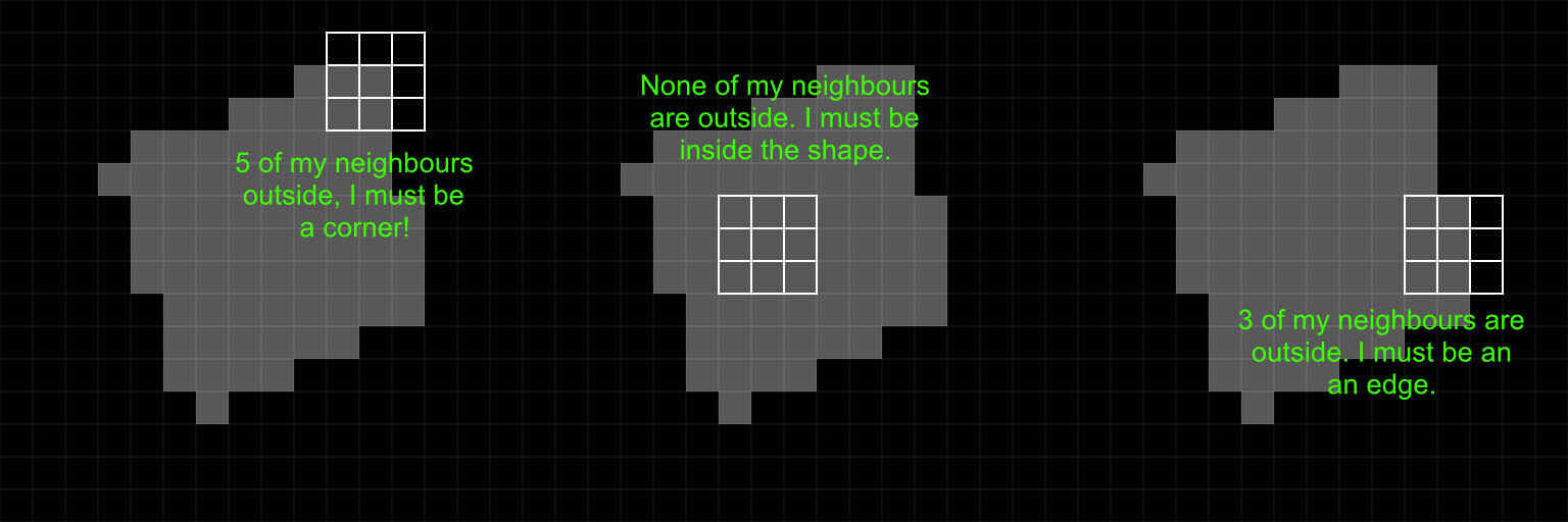
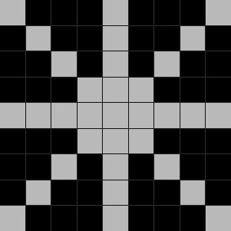
Below we have an image with a shape in it. A simple kernel might look like this, where the center cell is the pixel we are trying to calculate and the remaining cells are the 8 immediate neighboring pixels.

For each pixel in the kernel, we would run some math operations on it to calculate a final value for the center pixel. We could for example, add up all the pixel in the kernel and divide that by the kernel size to give us an average value of all the pixels in this 3x3 grid. Do that for all pixels in the image and we have implemented a simple blur.

You can visually think of the kernel looping over each pixel in our image, doing what ever calculation we want. Of course, our kernel could be any size and not necessarily looking at immediate neighbors either.

In reality, all pixels are calculated at the same time, rather then doing it one at a time like this, but I think the illustration can help to visualize what is happening.

So using this, how could we reason where corners are in a given shape? One approach, and the one I took, could be to count up how many neighboring pixels land inside the same shape and sum them up. Do this for all pixels and now you know where corners are in your image, pretty straightforward!

This is a very simple example, but if we had a bigger kernel with a larger image. The result gives us a gradient describing to what extent each pixel is a corner. With this gradient, we can apply various thresholds, levels, and tweaks to produce the outputs we want.

This is more or less how the whole node works. There are a ton of implementation details to solve but counting pixels inside the same shape is the high level approach.

Kernel Size and Python

Most image processing techniques require you to repeat a calculation a set number of times or across a given range of pixels. In programming this is achieved through the use of loops. However, the pixel processor has one major limitation, it doesn't support loops.

So for this reason, I create everything in the pixel processors with python and the API. We wont be going through that process here, since its way out of scope for this blog. But to give you an idea, I wrote a plugin with a set of functions for creating and connecting nodes.

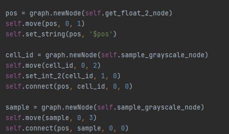
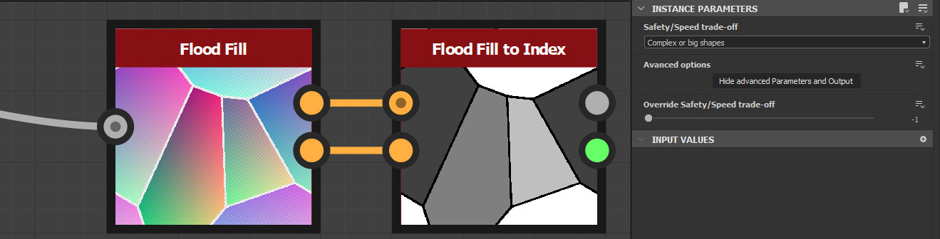
This way, I can easily iterate and use all of the Python toolkit, including loops. On the designer side, the plugin simply deletes everything inside the selected pixel processor node and rebuilds the node network for me.

Recall, the idea was to count all the pixels inside the kernel that reside in a shape. However, what would happen if we had two different shapes close together? We may inadvertently sample pixels from the other shape and mess up our count. We need a way to identify each shape independently.

The flood fill node has a 'Display advanced Parameters and Output' button, which you can use along with the flood fill to index node to output a unique number per shape.

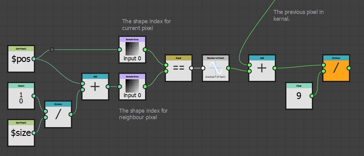
Then for each pixel in our kernel, we can check if the shape indices match. If they do, output a value of 1 otherwise output 0. Add that all up, divide by the kernel size and there is our value. This is what that could look like inside designer.

We also alluded to the need of having a big kernel in order to produce a sufficient gradient, so lets consider that a moment. In order for a pixel to describe how close it is to an edge, it needs to have seen that edge pixel to have been included in the calculation.

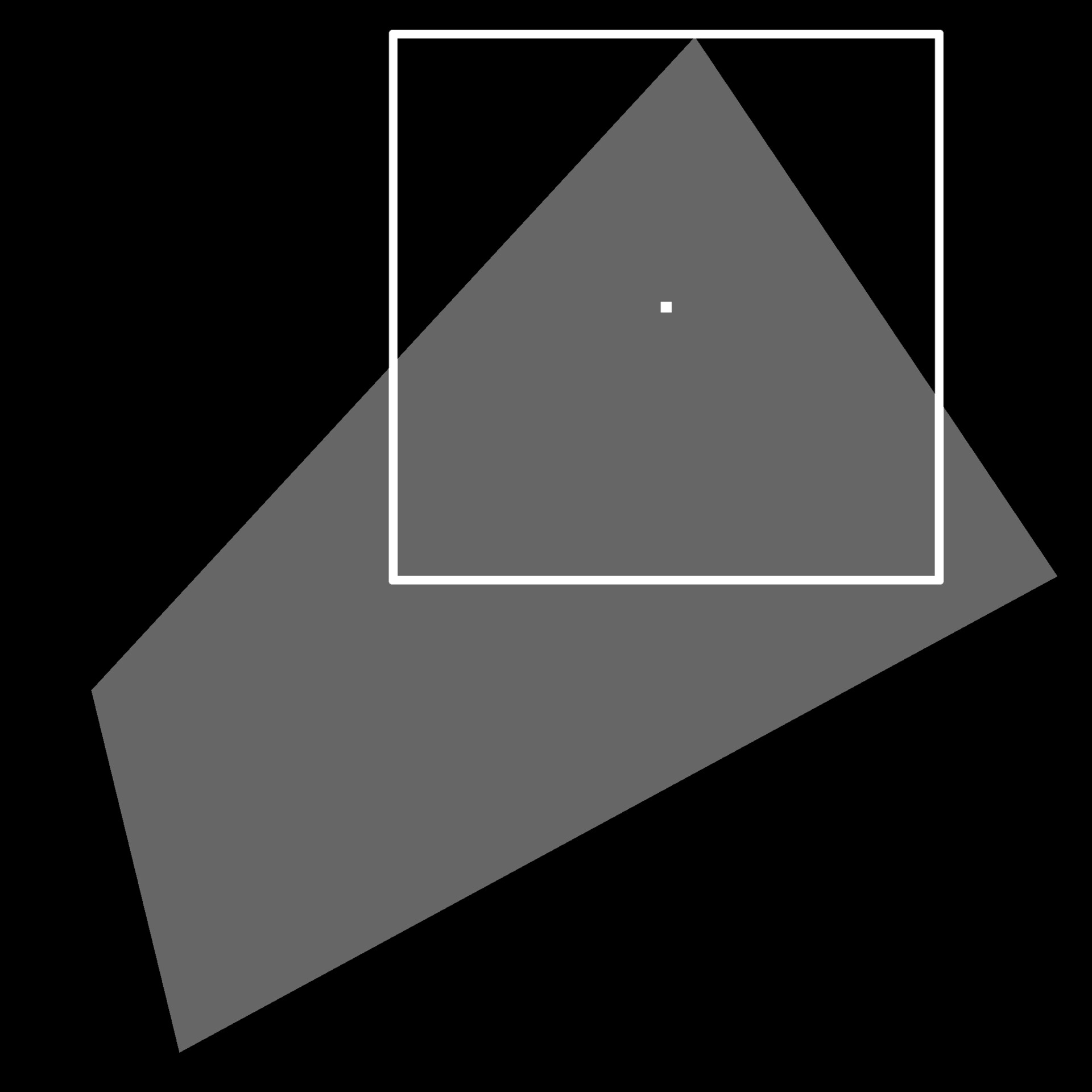
That's potentially a very pretty big kernel. In the image above, the shape covers nearly all of the texture and if we wanted the gradient to reach close to the middle of the shape, the kernel would need to be at least half the texture size. If this image was 2k, the kernel size could potentially be 1024x1024 or more. That's 4,398,046,511,104 total samples by the way (1024^2 pixels in the kernel per pixel in the image), which is obviously ridiculous.

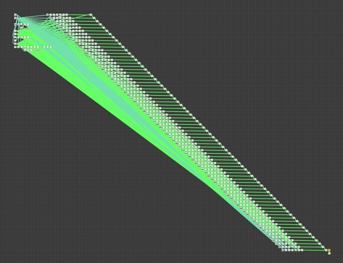
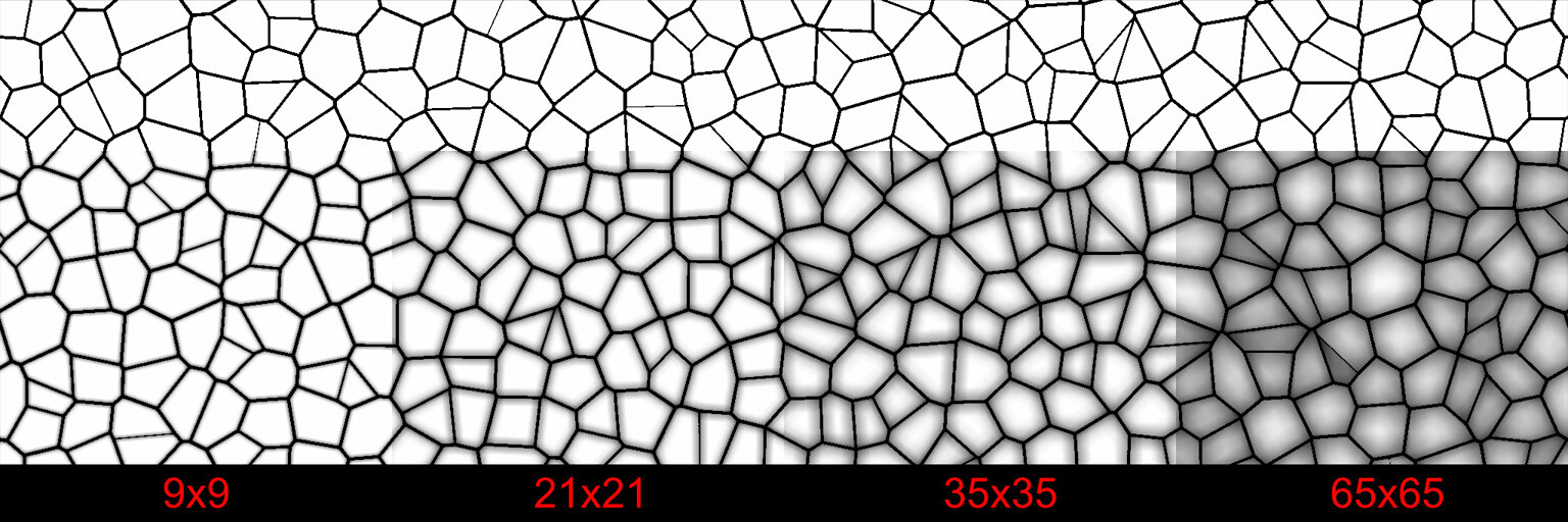
However, at this point I just wanted to test if the idea would work. So I took a typical use case and tried a few different kernel sizes.

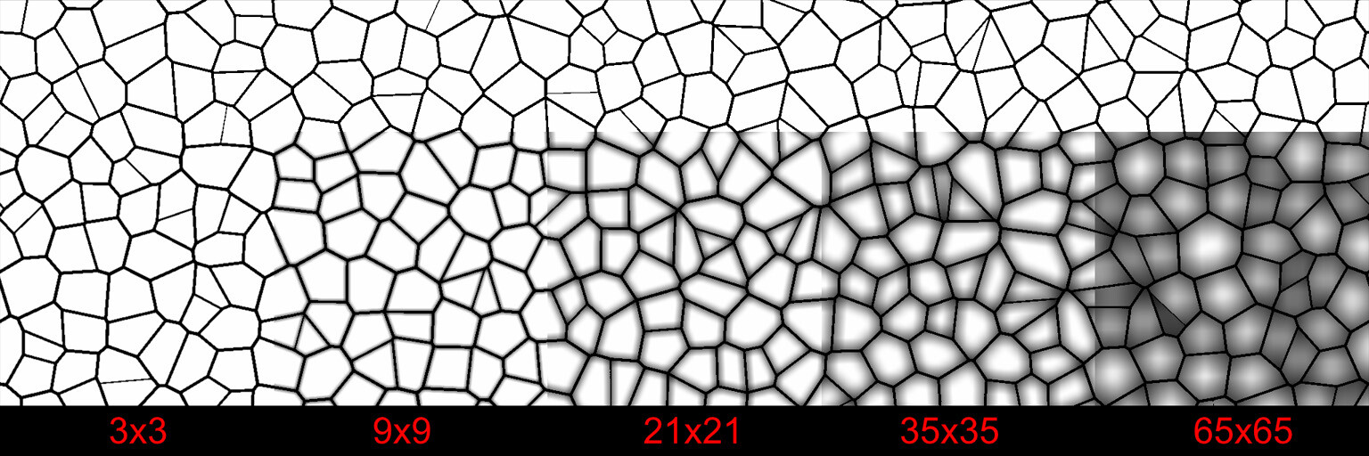
This somewhat confirmed the idea, but there are some glaring issues. The most obvious being performance. Even with a 65x65 kernel, this was 500+ ms on my machine and took several minutes to create the node.

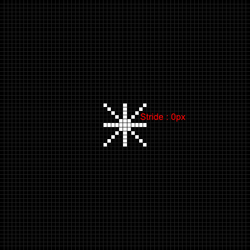
Perhaps we do not need so many samples to produce a good enough result. We could try sampling in a star shape instead, to see what difference that would make. This would reduce our sample count by over half.

The results are comparable and the performance was hugely improved. Even the mask output is perhaps a little nicer.

However, with the large gaps in the kernel now, there are some slight artifacts to the gradient and something we will talk more about in another post.

To address the issue of needing different kernel sizes for different shape sizes. My first thought was to define a stride between each neighbor so we could adjust the kernel to best fit the texture in hand.

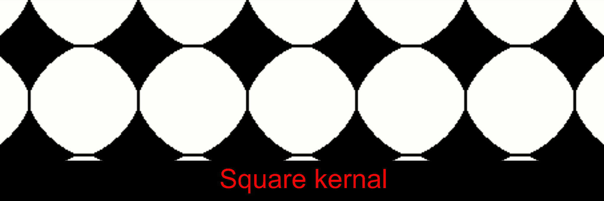
This certainly worked, but had the issue of very low sample counts producing prominent banding as the kernel size increases.

Furthermore, textures that feature large variation in shape size are handled poorly. Smaller shapes are quickly lost as the kernel covers the entire shape. Another topic we will talk a lot about in the following posts.

You may have noticed the corners are not very round and somewhat reflect the shape of the kernel. Notice here how squared off the corners are and how the star kernel has this slight pinch to it?

Well this is what the next part will be about, check it out here:
Part 2