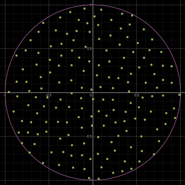
In the previous post, we had noticed how the corners were not very smooth and somewhat resembled the shape of the kernel. Maybe sampling in a circle rather than a grid might result in better rounding of the corners. If you haven't read part 1, I would recommend checking that out first as this is a direct continuation of that!
Circular Kernels
Another issue from our previous iteration, aside from the pinching, was how unintuitive the stride parameter was. It is quite difficult to mentally map what a stride value of means, when it changes depending on the kernel size and output size of the texture. So, perhaps we could define a maximum search radius relative to some constant value, like uv space, and then linearly scale our samples inside. A circular star shape of 8 sample points in concentric rings seems like a sensible place to start.
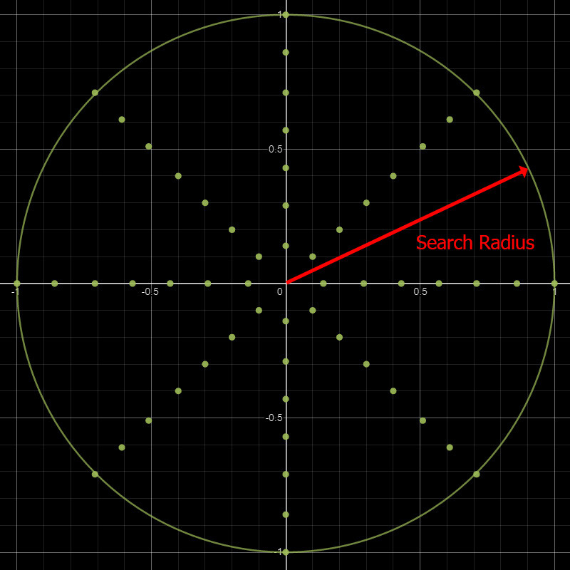
This allows us to adjust the kernel size independently of the sample count. In other words, we are free to add or remove more of these rings should we want more resolution without changing the overall size of the kernel.
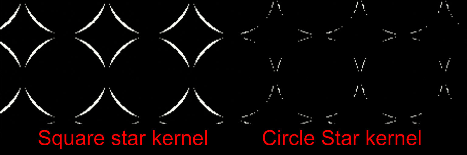
This confirmed our suspicion and resulted in a much smoother rounding. The image below shows the error from a perfect circle between the grid kernel and the circular kernel. More white means more error.
When viewing the sampling pattern on a graph, another problem becomes very apparent. Just how sparse the sampling becomes the further away we get.

Perhaps we should pick random points to sample within this radius instead? I have had trouble in the past with the random nodes inside designer being not very random. So instead of generating random sample points with those nodes, I precomputed the sample positions and brought them in as a float2 instead. Here is an example of what that could looks like.
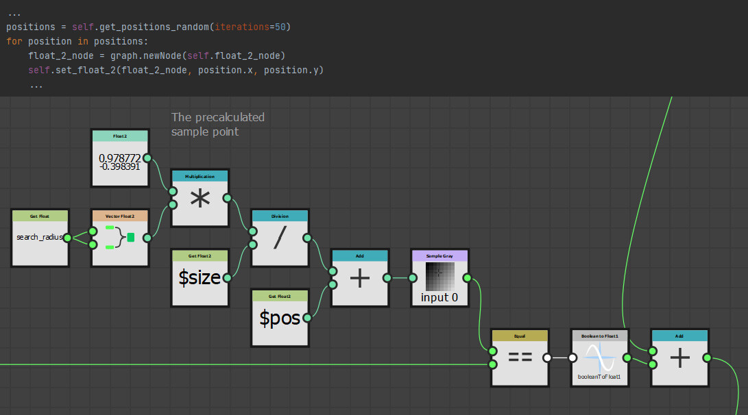
This as it turns out, this had a few benefits I did not expect, first of which was performance. Using float2 nodes is cheaper than calculating new coordinates at runtime. It also decoupled the node from the random seed slider. Meaning, the nodes output would remain the same regardless of the random seed value and if you have followed any of my previous work, you might know I am a big fan of this!
Perhaps the most useful benefit was having the sample positions available outside of Designer. Now we could paste them into a tool like Desmos to visualize exactly what the kernel looks like (This is how I create these graph images).
This was particularly helpful in debugging, as it is quite difficult to see what has gone wrong when creating these pixel processors through code.
Anyway, the results were quite promising!

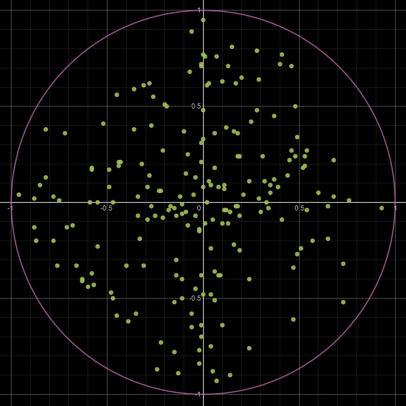
However, this introduced another rather awkward problem, the random points are... well random. Every time we iterate and rebuild the node the results are different. Some results are very wonky or lob sided. Indeed, it was a challenge just trying to generate this example image due to the randomness!
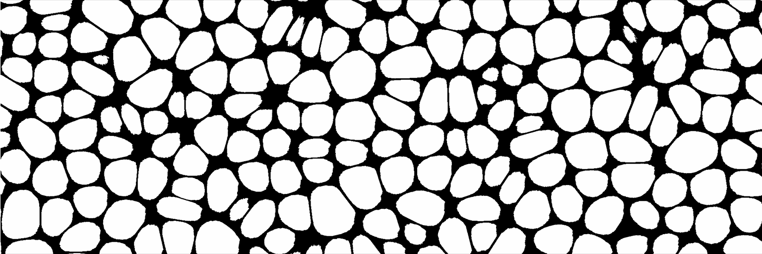
What we need is a more uniformly distributed pattern, something like a Poisson distribution. To be exact, its Poisson disk sampling we need, which is an algorithm to generate randomized points which are guaranteed to remain a minimum distance apart. The details of this algorithm is out of scope for this blog, but here is a nice breakdown should you want some further reading. Regardless, this is an example of the kernel with a Poisson distribution.
Now this is looking much better!
Since we are in python, generating these points was very easy. In fact, I found this implementation of it on github already, so there was no need to even write anything myself!
Here is a comparison between different builds of random sampling vs Poisson sampling. While the Poisson sampling is still random, the results are much more accurate and less variable between builds.

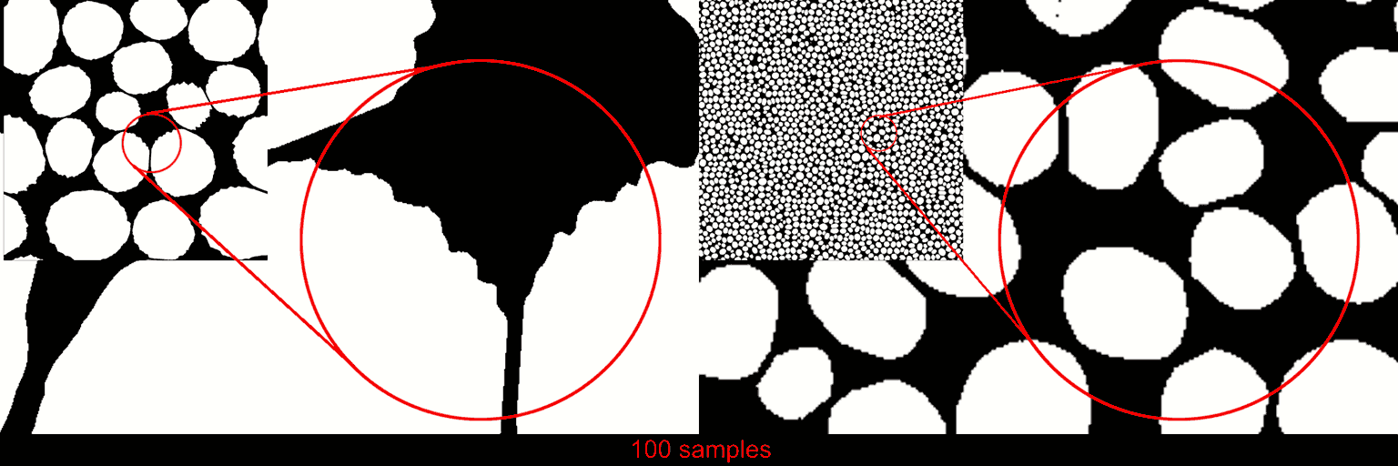
Up until this point, I had largely been testing on a 2k image and a fairly dense distribution of shapes. We still have a lot of artifacts when dealing with larger shapes though. I did do a lot of experimenting with smoothing these results (which we talk about below), but never did find an elegant solution to this problem. As far as I know, there just isn't a way around the issue with this sampling method. So, I decided the best approach was to expose a series of resolutions or sample counts to choose from. Ranging from 100, which is suited for these smaller shapes, up to 1000, to handle the large images.
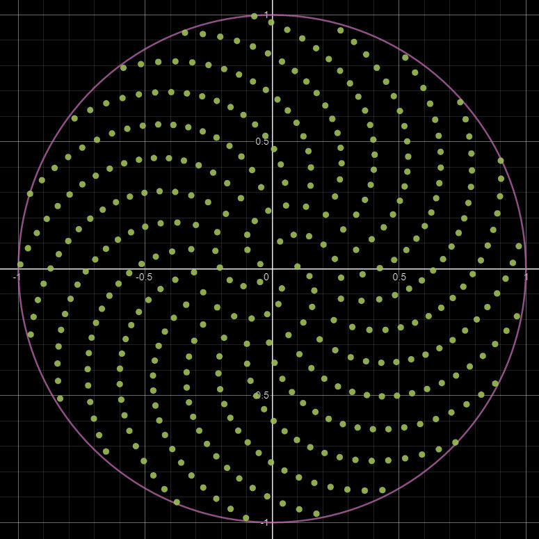
The results are cleaner, but only barely. The biggest benefit however is the sample points are not random, so every time we build the node, the pattern remains the same.
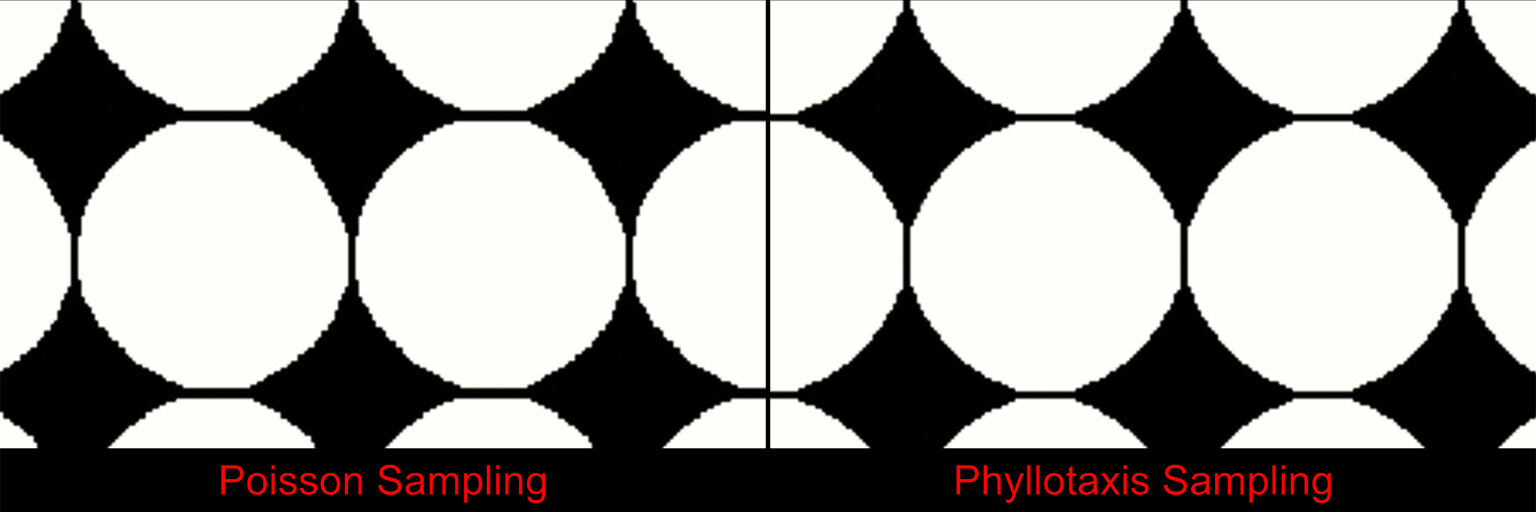
Phyllotaxis sampling it is then! And this is what the final release of the node is using.
Smoothing and Blurs
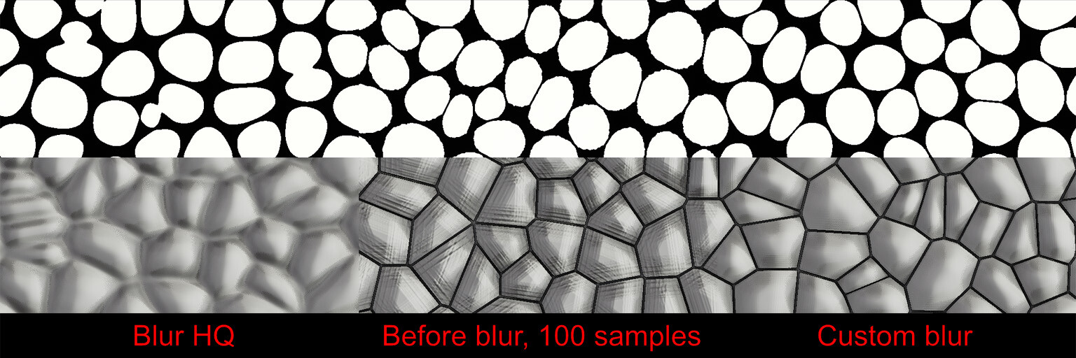
I mentioned a moment ago that I attempted to smooth out all these artifacts we have been getting, as an alternative to simply increasing the sample count. So what are these smoothing techniques? Well I tried all the typical nodes like blur HQ, non uniform blur, the suite of warps, but ultimately they all have issues relating to blurring across shape boundaries or losing the core shape. What we need is a custom blur that respects the individual shapes.
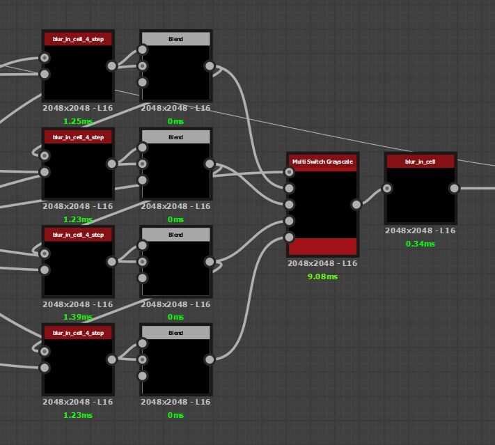
In fact, the example blur we described right at the start of this blog series is the implementation I went with. That is, looking at the 8 neighbors and averaging the result. However, we do a check first to see if the neighboring pixel is in the same shape. Exactly the same method as we did to calculate the corners. So we can try stacking a few of these and by a few, I mean a lot. I really did this many to even approach a smooth result.
This of course ballooned performance again.
Instead, let us try increasing the stride so we sample a little further out than the immediate neighbor. As it turns out, a stride of 4 was a very good compromise and we are able to cut this 400 pass monster by a factor of 100. Then to eliminate any artifacts left over from the larger stride value, a final immediate neighbor pass is done.
There is an interesting question with these blurs which might not be immediately obvious. If we sample a pixel outside of the shape, what value should we use?
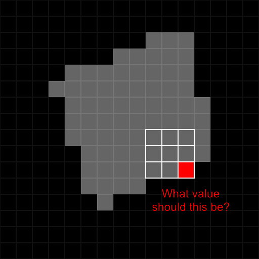 My first thought was to simply pass a value of 0, but as you see from the .gif below, that ends up completely loosing the original shape. Perhaps using the same value as the one we are calculating makes sense, the center pixel in the kernel? Or just ignoring the value entirely and only averaging those that are actually within the shape. These two ended up looking even worst!
The magic number turned out to be the center pixel * 0.9, which makes sense if you think about it. A slightly darker value is an approximation of the next value in the gradient, almost as though the gradient just continued to extend past the shape.
So, this is the majority of the node complete now. However, we still have a issue of varying shape sizes to solve. In the next post, we will discuss how we scale the kernel radius per shape and prevent the issue of smaller shapes disappearing altogether.
See you there!